An important task for the Institute of Marine Research is to investigate the dispersion and distribution of biological material and chemical substances in the ocean. This is managed best by utilizing dispersion models. We can in principle apply dispersion models to everything that passively drift with the ocean currents.
At the Institute of Marine Research, we use these models to simulate transport of eggs, fish larvae, salmon lice, virus and bacteria, nutrients, algae, radio activity, pollution, micro plastic and waste from mining activities. To be able to model particles realistically, we need to have access to output from a circulation model with sufficient resolution in time and space.
Dispersion models can be divided into two main classes: concentration-based and particle-based. Concentration-based (Eulerian) models solve an advection and a diffusion equation for concentrations, in the same way which is done for salinity and temperature in the circulation model. The alternative is particle-based (Lagrangian) models, where particles drift passively with the modeled current. Extra dispersion can be added to these particles by giving them an additional random displacement, which is commonly named random walk. Vertical processes like buoyancy, mixing and active migration can be added to the vertical displacement. We mainly use particle-based (Lagrangian) models at the Institute of Marine Research.
Transport of eggs and larvae
The Institute of Marine Research has been working with transport of eggs and larvae for several decades, involving a number of species. The general objectives for such analysis have been to study recruitment mechanisms and environmental impact on early life stages. The species that has been focused on so far are Northeast Arctic cod, Coastal cod, Norwegian spring-spawning herring, Polar cod, saithe, mackerel, eel, lobster and scrimp.
Particle tracking models are used to simulate transport of planktonic organisms that drift freely with the ocean current and has a limited ability to adjust their vertical position. Concentration-based models are mainly used for transport of nutrients and phytoplankton while particle-based models are used for eggs and larvae.
Particles representing eggs and larvae
Particle-based models are particularly well suited for modeling transport of eggs and larvae, and these models do not require large computational resources. Each particle has its own identity, meaning we choose where it is released and store all information along its pathway including the ambient environment and exact position. This makes it for instance easier to calculate potential overlap with pollution in exposed areas. The particle concept is also suitable for individual-based biological models that includes individual growth and survival, which depends on for instance temperature and food availability.
Vertical distribution determines the transport
Previous studies have shown that determining the vertical distribution of eggs and larvae has a significant impact on the horizontal transport and how the environment is experienced by the particle (egg/larvae). Since the vertical distribution of eggs is depending on their buoyancy while the larvae can migrate vertically, it is convenient to handle these two stages separately. This can easily be done by allowing the particle to move horizontally according to the advection model, while the added vertical movement for the particle vary between the egg and larva stages. The egg buoyancy depends strongly on the density difference between the egg and the surrounding waters and should be moved accordingly, while the larvae for most species can migrate actively typically in the upper 50 m of the water column. The latter is hard to parameterize in the model and must be supported by larvae experiments in sea water.
A possible cause of active vertical migration for fish larvae is the presence of prey and predators. By swimming upwards in the water column, the larvae will be able to see their prey better and at the same time they are more exposed to predators than if they swim deeper. Available observations indicate that larvae perform diurnal vertical migrations to find prey and avoid predators, however there are uncertainties associated with these data and it varies between species. More observations of larvae co-located with observations of prey and predators will be fundamental to fully understand these processes.
Disease dispersion
Salmon lice begin life with larval stages hatched directly into the water masses and develop through three non-feeding planktonic stages: two nauplius stages (non-infective) and the infective copepodid stage. If the lice larvae cannot locate a host fish in time they will die from starvation or predation. During these early life stages the larvae can position themselves vertically in the water column, but otherwise they drift freely horizontally with the water currents.
Information on the number of hatched eggs from the salmon farms is crucial for the quality of model estimated salmon lice infection pressure. Based on the temperature and number of adult female lice per fish (reported weekly by the fish farms), and the estimated number of fish in the farms (reported monthly), the number of nauplii released into the water masses per hour from each farm is calculated. This information is fed into a dispersion model that estimates the position of the salmon lice larvae as a function of the oceanographic conditions (currents, temperature and salinity).
The salmon lice infection pressure shown at lakselus.no is estimated in real time, thus the number of fish at the farms might be inaccurate in cases where fish are slaughtered but have not yet been registered in the database. The model estimates are therefore calculated in retrospect when more accurate registrations from the farms are available, before the estimated salmon lice infection pressure are use in management assessments.
Organic material from fish farms
Within a large fish farm there are several hundred thousand fish swimming around, being frequently fed. The majority of the fish feed is eaten, but a certain fraction passes through the cages and sinks towards the bottom. Some of the excess feed is eaten by wild fish, the remaining part settles on the sea floor beneath the farm, as does the fish feces. Here the organic material is eaten by benthic animals like crabs, sea porcupines and starfish, or bristle worms and microorganisms living in the sediments. Our models can tell us which areas around the farm are affected by the organic waste.
Large amounts of organic material can change the bottom fauna, as opportunistic species begin to multiply and replace native species in the area. In regions with weak water circulation, the oxygen levels may be depleted as a consequence. Occasionally, therapeutic agents are added to the fish feed, some of which may enter into the fish feces and be harmful to benthic species. These are some of the reasons why fish farms should be placed at a distance from sensitive habitats.
In order to know the range of influence from fish farm organic waste, we use particle tracking models coupled with current circulation models. The particle tracking model contains a large quantity of virtual particles that are released from the farm, with individual sinking velocities based on studies of physical feed and fecal particles. The virtual particles can also be resuspended if the local currents are sufficiently strong. Resuspension events are most likely to occur in shallow waters under the influence of strong winds and waves.
The particle tracking models are used to study the ecological consequences of particulate effluents both around single farms and in a larger area. There is ongoing research on the influence of organic material and in-feed drugs on benthic fauna and other species. The models provide a means to understand the practical implications of this knowledge, for instance how large buffer zones should be established around sensitive habitats to protect from harmful effects of fish farms.
Dispersion of plastic
Marine plastic can roughly be divided into two categories that will behave very different in the water column: buoyant plastic that consists of polymers lighter (less dense) than seawater that will float on surface if undisturbed; and sinking plastic that consists of polymers heavier (more dense) than seawater sinking out of the water column. Worldwide 60% of plastic produced today consists of polymers buoyant in seawater. The relative density of the polymer to seawater will to a large degree dictate how fast the particle will float to the surface or sink out of the water column, which has large consequences for the dispersal potential of the plastic particles. Furthermore, plastic is also divided into size classes where microplastic consists of particles and fibers not easily observable by the naked eye where special microscopes or chemical methods are used to distinguish the particles. Because more drag is exerted on particles when surface to volume ratios is large (i.e. Stokes law in laminar flow) typical of smaller particles the terminal velocity of large particles will be higher and the larger particles will attain their surface or bottom maximum faster. A further complicating factor for the placement of the polymer in the water column is the added weight of biofouling, which may even transform an otherwise buoyant particle to a sinking particle, or the particle may become neutrally buoyant more akin to a pelagic fish egg. Turbulence for example from breaking waves will also create more than enough motion to stir the otherwise buoyant particle far down the upper mixing layer. Fragmentation of plastic particles due to UV radiation or other mechanical stress will also necessarily have an impact on all these factors. A large diversity of marine bacteria that may utilize hydrocarbons as base for nutrition has also been found on marine microplastic, which over time also may affect particle size and degradation.
All the theoretical considerations reviewed above on the physical properties of plastic polymers and their interaction with seawater are all working hypothesis, that may or may not hold true in real-life. Research on plastic in the marine environment is a relatively new field, where many new discoveries will shift our understanding in either way. For example, why do we find plastic particles that in theory should sink to the bottom floating in the middle of the Polar basin? Or a buoyant polymer particle on the bottom of a Svalbard fjord? And how far will a polyester fiber from your laundry discharged with the sewer into the ocean be dispersed by the ocean currents? These questions we apply dispersal models to try to find the answer to.
Dispersion of chemicals
Sea lice has been identified as the most important obstacle to further growth of the aquaculture industry. Several methods are being used to remove lice from the fish, one of these methods is in-cage bath treatments. In this process, the cage is enclosed by a tarpaulin and anti-sea lice drugs are administered directly to the water. After treatment the tarpaulin is released, and the chemicals are diluted and transported with the ocean currents. We use simulation models to gain an understanding of the dilution rate and how fast the chemicals are transported before being diluted to environmentally safe concentrations.
The dilution process is turbulent and happens over a large geographical area. It is therefore difficult to obtain a correct impression of the concentration distribution in the ocean using physical water samples. Computer simulations, on the other hand, are very helpful. Both field-based and particle-based models can be employed, but one drawback of field-based models is that they often overestimate dilution – so-called numerical diffusion. The problem is solvable, but one has to be aware of the model’s weakness and use it correctly. At the Institute of Marine Research we have instead used particle tracking models to simulate chemical releases from fish farms.For å vite hvor langt påvirkningen fra organisk materiale strekker seg fra oppdrettsanlegget, bruker vi partikkelspredningsmodeller som er koblet til strømmodeller. Spredningsmodellen inneholder en stor mengde virtuelle partikler som slippes fra anlegget, med individuelle synkehastigheter som er basert på studier av fysiske forpartikler og fekalier (avføringsklumper). De virtuelle partiklene kan også virvles opp igjen fra havbunnen dersom den lokale strømmen er sterk nok. Slike oppvirvlingsprosesser (resuspensjon) forekommer oftest på grunt vann under kraftige vindforhold og høy bølgeaktivitet.
Small release volumes are diluted more quickly than large volumes. The dilution rate is also determined by the local ocean currents near the fish farms. Whether a concentration is harmful or not depends on the agent used, the non-target species under consideration and the exposure time. These toxicity data are determined by laboratory experiments. If we also have a model of the organism’s migration pattern, it can be coupled with the dilution model. This allows us to predict the risk of an organism coming in contact with harmful concentrations of the chemicals. For instance, many species live close to the sea floor, and thus have a reduced risk of exposure to large concentrations of bath treatment drugs. An important exception is hydrogen peroxide which is heavier than water. In wintertime, when the density is close to homogeneous within the entire water column, hydrogen peroxide from a tarpaulin bath treatment operation can sink towards the bottom and spread along the sea floor.
An alternative to tarpaulin bath treatments is well boat bath treatments, which has a smaller ecological footprint. First, the release volume is often less than a corresponding tarpaulin treatment. Secondly, the wastewater is released gradually from the well boat while moving, which accelerates the dilution process. Thirdly, a well boat may transport the treatment water away from sensitive areas before being released.
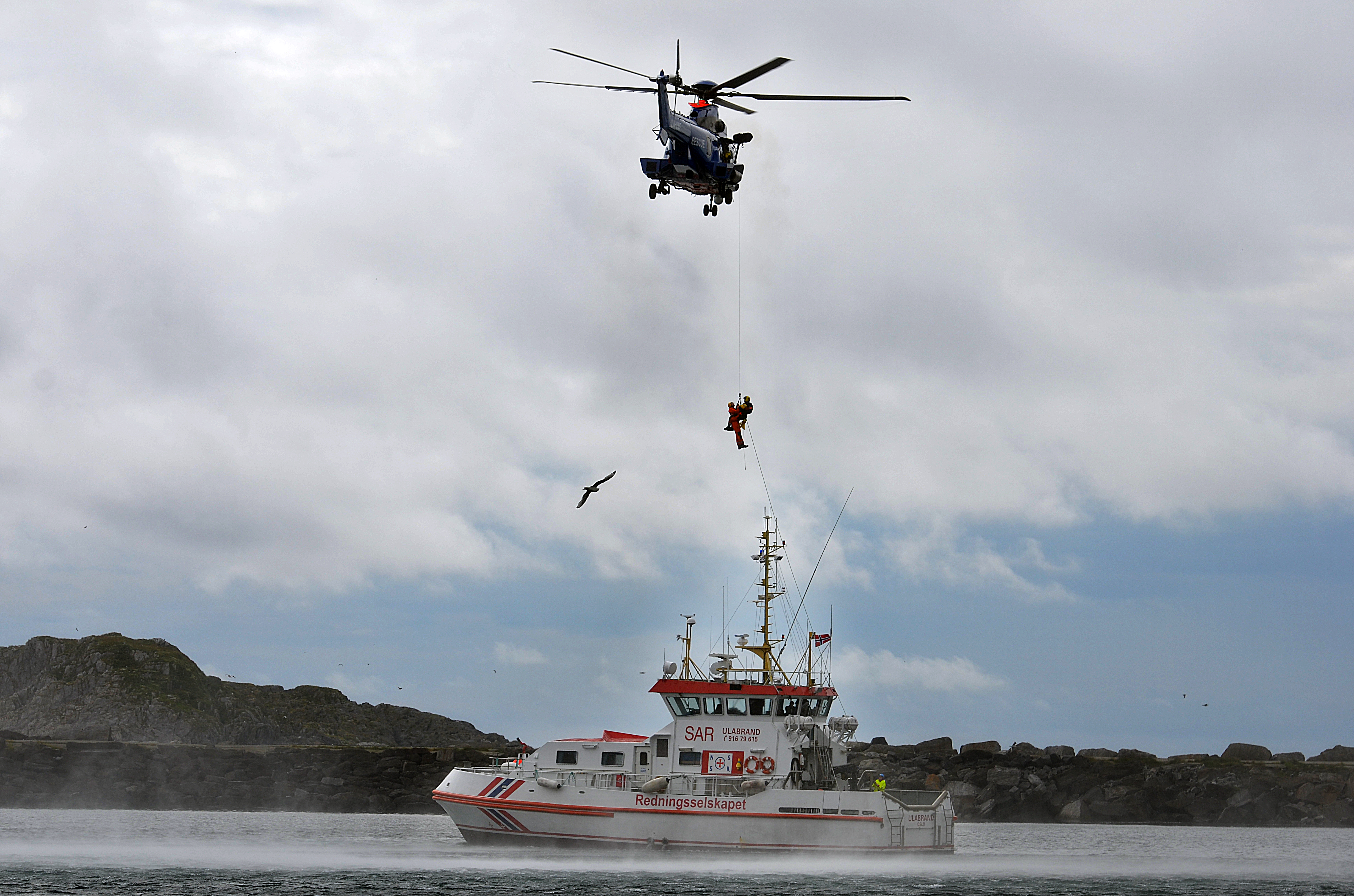
Search and rescue
Picture from a rescue demostration in Sørvær.
Photo: Gunnar Sætra / IMR
When the alarm goes off, for example a person has ended up in the sea, the Joint Rescue Coordination Centres (JRCC) will lead the rescue operation. JRCC utilizes model output from the Norwegian Meteorological Institute (MET-Norway) to visualize the most likely drift forecast and potential range. But if the accident happens near land, along the coast or inside a fjord, we need to simulate the current conditions using more details and higher precision.
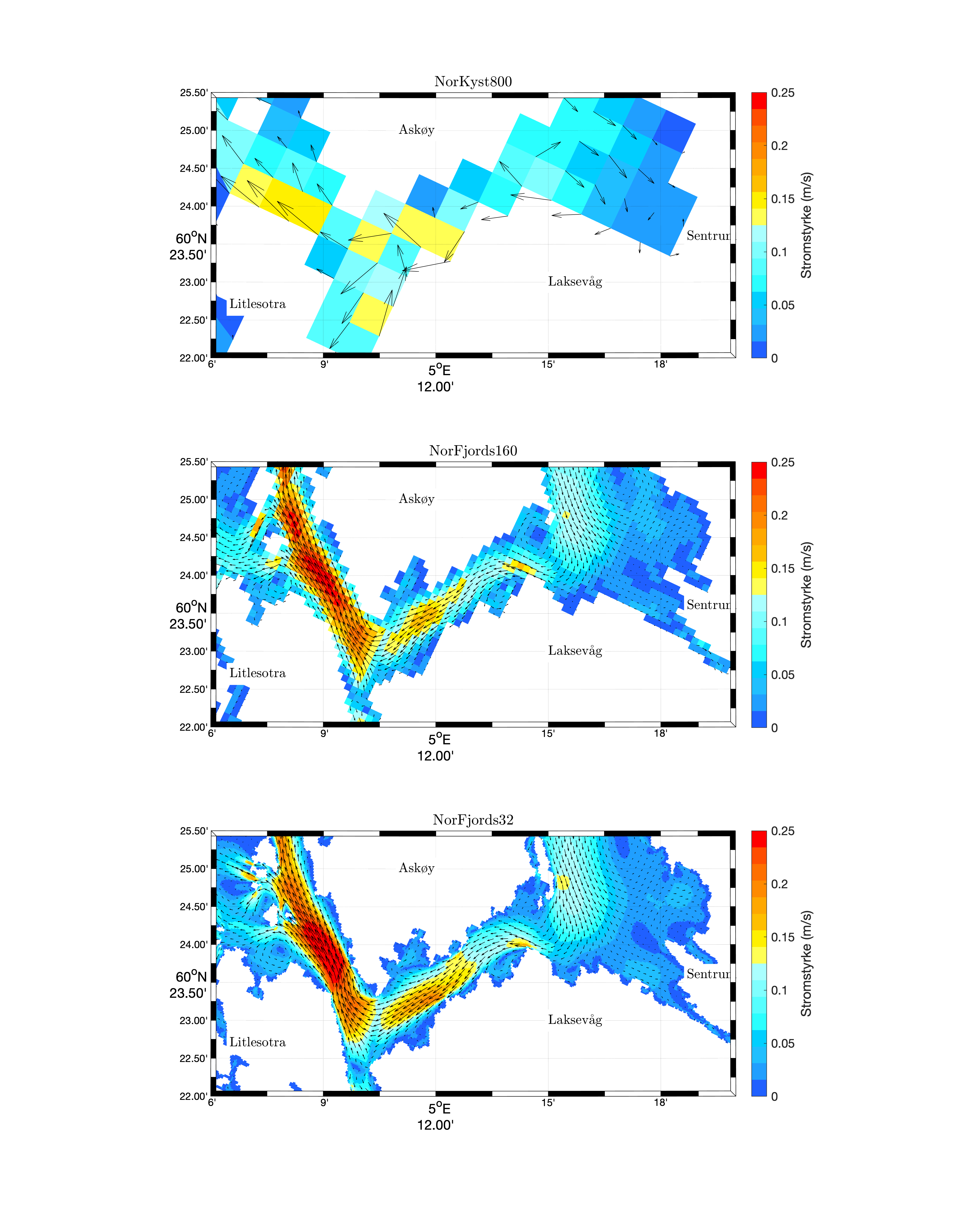
When the rescue operation goes from a search operation to a search for presumed dead, the Institute of Marine Research (IMR) has a national model system that can simulate ocean currents anywhere along the coast with a resolution down to 160m x 160m. This fjord model is in principle similar to the forecast model NorKyst800 run at MET-Norway, but it is so computational demanding that it is difficult to produce daily forecasts for the entire country. When you are able to estimate the current conditions at such a detailed level as you can perform with a high-resolution fjord model, you can with significantly greater accuracy give advice on where to search when the search area is in more narrow waters. IMR has also experimented with fjord models using 32m x 32m resolution for special detailed waters, but these are very time consuming, both related to establishing and computer processing.
There are two ways these detailed ocean current information can be utilized in order to indicate possible pathways and spread potential from a specific location point. One option is to demonstrate typical current conditions at the site, based on statistics. We possess long model archives ready to generate such statistics. An alternative possibility is to run a full ocean current simulation for the actual place and time, and this allows us to estimate the most likely direction of currents during the relevant hour and day. Such a modelling exercise takes at least 24 hours to complete.
A significant challenge with such simulations is that one often does not have information about the depth for which the drift should be calculated. Using Byfjorden outside Bergen as an example, an object or person will normally drift westward toward Litlesotra as the surface currents tend to go westward more often than in the opposite direction. However, if the person sinks deeper, then compensating current flows in the opposite direction, and the deep-water drift will be altered relative to surface drift implying a completely different search area. Such vertically separated current patterns are very normal for Norwegian fjords and straits. The current goes one way in the surface, and you may have currents in the opposite direction further down. It is therefore essential to be able to indicate how deep a person or object that falls into the water sinks. But you rarely have info about how deep someone has ended up. The drift pathways must then be calculated for several depths to include different possible scenarios, and these estimates may give completely different search areas.
If a deceased person has been found, we can in theory also utilize the same modelling system to track a pathway back in time to e.g., estimate where the incident occurred. Such backtracking is difficult to perform precisely, but some indications can usually be obtained.
IMR has a close and good collaboration with its oceanographic research colleagues at MET-Norway to achieve better resolution of the operational models which they operate. Hopefully JRCC then in the near future can have access to sufficiently resolved current models for more detailed information on search areas in fjord regions.
These three surface current maps cover an area encompassing Byfjorden west of Bergen (Sentrum), using different model resolutions. The upper panel shows results from NorKyst800, and that is the best resolved operational forecast model that JRCC currently has access to from MET-Norway. For Byfjorden we need more details on local conditions. The middle model has 160m x 160m between each calculation grid cell, and it corresponds to the national model system that IMR has at its disposal and can produce results from. The lower one has a resolution of 32m x 32m and is a test version of a model with extra high resolution.