Oppfølgingsstudie av fiskeforekomster ved Hywind Tampen havvindanlegg under konstruksjon og tildig operasjonell drift
Målet med toktet var å følge opp forsøkene som ble gjennomført i 2022 før utbygging av Hywind Tampen startet. I mars 2023 da toktet ble gjennomført var syv av de elleve planlagte turbinene i drift. Som i 2022 var forsøkene basert på en gradientfangststudie. I forsøkene ble kommersielle torske- og seigarn brukt på forhåndsbestemte stasjoner med økende avstand til vindkraftverket. Fangstene ble analysert for informasjon om artssammensetning og tetthet, modningsstadie, kondisjon, størrelse og diett og hvordan disse varierer med avstand til vindkraftverket. I tillegg ble det samlet inn akustiske data.
Høyest antall arter ble registrert i de grunnere områdene lengst unna vindkraftverket (15 -18 nm). De vanligste artene som også er av kommersielt interesse var lange, lysing, sei, torsk, lyr, hvitting og hyse. Med unntak av sei ble disse hovedsakelig fanget i de grunne områdene. I motsetning ble bruskfiskarter hovedsakelig fanget i de dypere områdene nærme vindkraftverket. Resultatene var like de i 2022, bortsett fra noen forskjeller i dybdefordeling av fisk. I de akustiske dataene ble det ikke registrert noen fiskestimer, men lag av svake ekkoer fra plankton og mesopelagiske fisk. Dårlige værforhold resulterte i få prøver fra de dypere områdene nærme vindkraftverket. Derfor er de statiske analysene usikre og man må være forsiktig med å overtolke resultatene.
På dette toktet og i 2022 er det blitt samlet inn biologisk data om bunnfiskarter i Hywind Tampen området med høy oppløsning. Med videre datainnsamling vil det være mulig å undersøke mulige effekter av flytende havvindkraftverk på marine økosystem.
Sammendrag
The aim of the cruise was to follow up the pre-construction studies in Hywind Tampen in 2022. In march 2023, when this cruise was carried out, seven of the eleven planned turbines were in operation. As in 2022, the experiments were based on a gradient fish capture study using bottom gillnets at pre-determined stations. The catches were sampled and analysed to obtain information about species richness, abundance, maturity stage, sex, condition and diet and how these vary with distance to the windfarm. In addition, acoustic data were collected.
The highest number of species and the highest abundances were registrered in the shallow areas furthest away from the windfarm (15 -18 nm). The most common species, that also are of commercial interest, were ling, hake, saithe, cod, pollock, whiting and haddock. Elasmobranch species were mainly caught in the deeper areas closer to the wind farm. The results from this cruise were similar to those in 2022, except for some differences in depth patterns in fish abundances. No fish schools were registered in the acoustic data. However, layers of weak scattering organisms were present in most of the transects. Poor weather conditions resulted in a small sample size for the deep region in this survey. Therefore, the power of the statistical tests for differences with depth or distance is low.
This and the 2022 cruise have collected valuable fine resolution biological data about the demersal fish species in the Hywind Tampen area. With continued sampling these experiments can reveal potential effects of the installation of Hywind Tampen wind farm on the marine ecosystems.
1 - Introduction
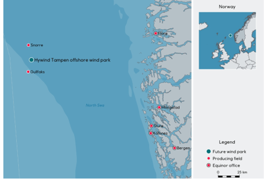
Hywind Tampen floating offshore wind farm consists of 11 turbines with a total capacity of 88MW. The wind farm is estimated to meet about 35% of the annual electricity power demand of Snorre and Gullfaks oil and gas platforms (https://www.equinor.com/energy/hywind-tampen). The wind farm is located in the northern North Sea, on the western edge of the Norwegian trench, at 250-300 m depth (Figure 1). The area coincides with a traditional bottom trawl fishing area for saithe and more sporadic trawl and purse seine fishing grounds for pelagic species (Directorate of Fisheries, www.fiskeridir.no). Nearby, in the shallower areas west of the wind farm, Danish seine and gillnet fisheries target mixed demersal species. The overall aim of the cruise was to collect data that contribute to long-term investigations on the effects of floating wind farms on marine ecosystems, with a main focus on commercially important demersal fish species.
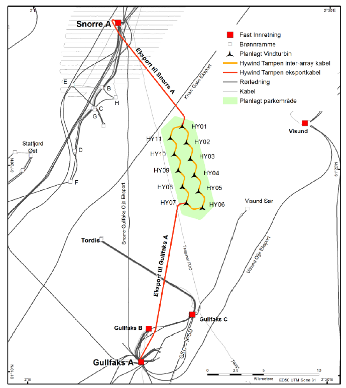
In March 2022 a research cruise was carried out in Hywind Tampen to map demersal fish distribution before construction of the wind farm started (de Jong et al., 2022). In March 2023, 7 of the planned 11 turbines were in operation (Figure 2). A follow-up survey was carried out to investigate fish distribution during construction and in an early stage of operation. The two surveys were at the same time of the year and using the same survey design, fishing vessel and fishing gear. The experiments were based on a gradient fish capture study using bottom gillnets at pre-determined stations at increasing distance from the windfarm (Methratta, 2021). The aim was to describe how species richness and abundance, as well as length distributions, diets and maturity stages of the most common species (cod, ling, haddock, hake, pollock and saithe) change with distance to the wind farm.
Figure 1 . Map of the North Sea and the Norwegian Sea showing the location of Hywind Tampen. Map by Equinor (Equinor.no)
Figure 2 . Location of the wind turbines in relation to the oil platforms on Gullfaks and Snorre. (Map re-used from Equinor 2019 Hywind Tampen PL050 – PL057 – PL089 PUD del II – Konsekvensutredning). Turbines HY02 – HY05 were not in place during the cruise.
2 - Methods
The experiment was conducted between 20 – 27 March 2023 with the chartered fishing vessel MS Nesejenta (Table 1). Wind speeds in the survey period ranged between 4 and 15 m-s and current strengths near seabed ranged between 0.1 and 0.7 knots (Table 2). The sea state was moderate to rough with wave heights ranging from 1 to 4 m.
Name
Affiliation
Role
Maria Tenningen
Institute of Marine Research
Cruise leader
Kate McQueen
Institute of Marine Research
Researcher
Vidar Fauskanger
Institute of Marine Research
Technician
August Fjeldskår
Nesefisk AS
Captain
5
Nesefisk AS
Crew
Table 1 . Cruise participants
Date
Wind speed (m s-1)
Wind direction
Current speed (kn)
Current direction
Sea state degree
21.03.2023
5 - 14
SE
0.2 – 0.6
S
4 – 5
22.03.2023
11 -14
S
0.3 – 0.5
S
5
23.03.2023
4 – 8
SE
0.2 – 0.7
S
4
24.03.2023
8 - 16
NE
0.1 – 0.2
W
-
25.03.2023
13 - 15
NE
0.3 - 0.4
E
5
26.03.2023
10 - 14
NW
0.2 – 0.3
-
-
Table 2 . Weather conditions were registered at each station when the nets were set and hauled in. The data are presented as daily range in wind and current speed and the main direction. Sea state was determined based on visual observations and using the “international sea and swell scale”
2.1. Vessel details
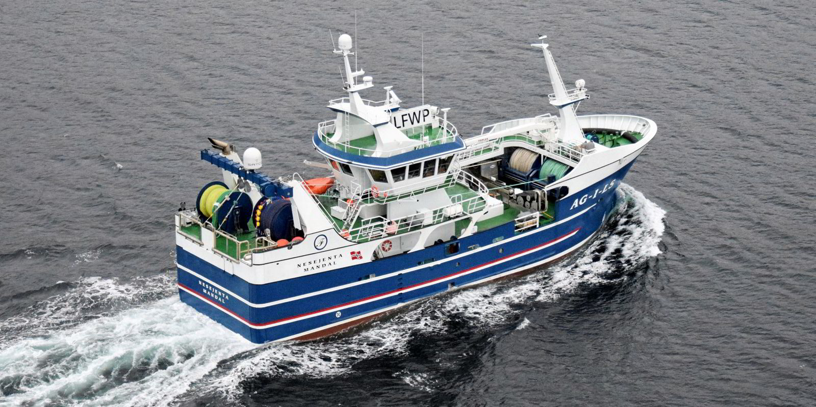
The fishing vessel Nesejenta (AG-1-LS) conducts commercial fishing for demersal fish in the North Sea, the Norwegian coast, and the Barents Sea (Figure 3). The vessel is equipped for fishing with gillnets and Danish seine. It was built in 2020 and is 35.3 m long, 9.10 m wide and has a gross tonnage of 499 tonnes.
The vessel was equipped with a current meter and fish finding equipment including a Furuno FCD 1900 echosounder and a WASSP multibeam sonar. In addition, the vessel has an Olex mapping system that was used for navigation and planning of fishing operations.
Figure 3 . M/S Nesejenta a commercial gillnetter / Danish seiner was chartered for the experiments (photo: Frode Adolfsen, Fiskeribladet.no) .
2.2. Fishing gear
In the experiments, we used commercial saithe (74 mm half mesh size) and cod (90-93 mm half mesh size) gillnets. The nets were arranged in 5 fleets of 60 nets each. Each fleet contained 20 saithe, 20 cod and 20 saithe nets. The nets were about 28 m long and 50 meshes high. All fishing operations were carried out by professional fishermen. The fishing vessel’s own quota was used, and all catches were stored on ice and sold after the cruise.
2.3. Experimental design
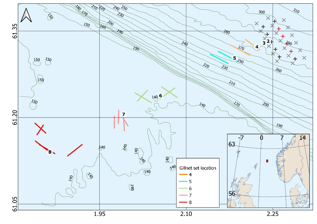
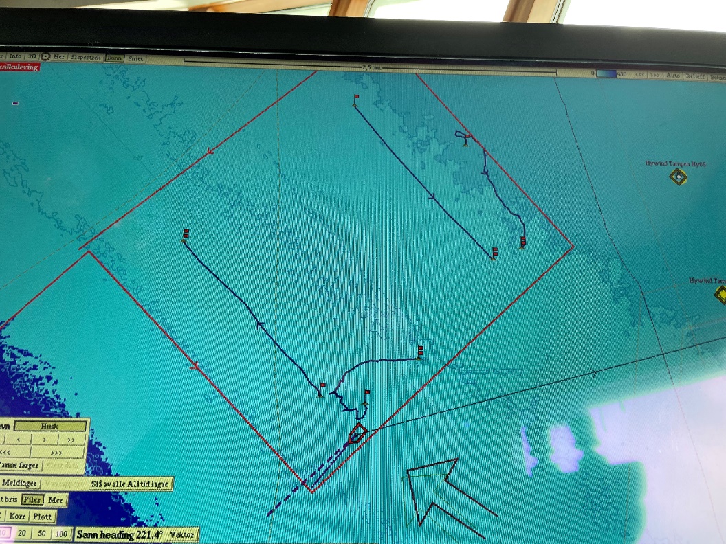
The experiments were based on a gradient fish capture study with pre-determined gillnet stations at increasing distance from the windfarm. The same design was used in the 2022 experiments (de Jong et al., 2022). For the 2022 experiments, 8 stations were defined between 0 and 18 nm in a south-western direction from the wind farm. This year the first station 100 m from the middle turbine (HY09, Figure 2) could not be sampled as it was inside the 500 m safety zone. The aim was to set all five gillnet fleets each day and have 3 – 4 replicates from stations 2 to 8 (Figure 4). However, due to poor weather conditions (Table 2) we only managed to set all five fleets on the first day. The following 5 days we set 0 – 3 fleets per day (Table 3). The conditions were challenging, with wind speeds mainly above 10 m-s, a sea state between 4 and 5 and bottom currents ranging between 0.2 and 0.7 kts (Table 2). In stations 2 - 5, on the slope, the nets did therefore not properly attach to the soft seabed. We experienced that the nets twisted and drifted in an northeastern direction towards the wind farm. An AIS tracker attached to some of the nets showed that the nets drifted about 0.5 nm per hour (Figure 5). To avoid the risk of nets drifting inside the wind farm and entanglement in chains or cables of the floating turbines no nets were set in stations 2 and 3.
Figure 5 . Screendump of the Olex map showing how the gillnets drifted in the stations near the windfarm.
A total of 17 catches were conducted, with 4-5 replicate catches per station in the shallow region, and 2 replicate catches per station in the deep region (Table 3, Figure 4). All fish were brought on board and samples were taken for the first twenty fish for each species in each catch. Fish were measured to the nearest cm and weighed to the nearest gram up to a maximum of twenty fish per catch. For hyse/haddock, lange/ling, lysing/hake, sei/saithe, lyr/pollock and torsk/cod, we also took stomach samples and muscle samples (for stable isotope analyses) of the first five fish at each location (Table 4). Some fish had inverted stomachs due to the pressure change during hauling, these stomachs were not collected. Especially in the catches in the deeper waters, fish were eaten by sea lice while caught in the nets. In such cases a measurement of length was often still possible, but the weight was not measured.
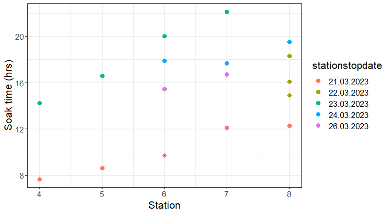
Weather conditions and practical considerations prevented a fully randomized design. However, there was no significant relationship between soak time and distance to the wind farm, calculated as the distance in kilometres from the midpoint of the set position to turbine 9 (61.33N, 2.25E) (F1,15=4.25, p=0.06, R2=0.17) (Figure 6).
Figure 6 . Soak time, as time from setting to hauling, at the different locations (4 = closest and 8 = furthest from the planned location of the wind farm). Colour of points indicates date of hauling.
2.4. Statistical Approach
While the figures shown in this report represent the data per station, the statistical analyses were done using linear models with the distance to the wind farm site (in kilometres) as a continuous explanatory variable. This distance was calculated from the midpoint of each gillnet (set position) to the closest turbine 9 (61.33N, 2.25E) (See Table 3). To separately assess the effect of the distance to the wind farm site and the effect of depth on species richness the data were split into two depth categories (deep: station 4-5 and shallow: station 6-8). Serial 57910 (station 5) was excluded from statistical analysis, due to twisting of 2/3 of the nets in the link. Thus, the analyses were conducted using data from 3 samples from the deep region, and 13 from the shallow region. The small number of samples from the deep region results in low power of the statistical tests comparing depth categories. Distance to the wind farm analyses were conducted only using samples from the shallow region.
Poisson GLMs were used to assess whether species richness varied with distance from the wind farm site within these depth categories. In addition, a model was fitted to test for a difference in species richness between the two depth categories. Soak time in hours (log transformed) was included as an offset in all models.
The most abundant species caught, which are also of commercial interest, were ling, hake, saithe, pollock and cod. To assess how abundance of these key species varied along the transect, the same modelling approach as described for species richness was used. Overdispersion in Poisson GLMs was dealt with by correcting standard errors using a quasi-GLM.
Sample sizes and number of spawning fish were too low to conduct statistical tests on proportions of spawning fish.
Linear models were fit to the length and condition factor data to test whether size and condition factor of fish varied between depth categories and distance to the turbines. Subsamples were used to predict the length and condition of the total number of fish in the catch. This was done by including raising factors as weights in the linear models.
Station
Serial nr.
Repl. nr.
Date (start)
Time (start, UTC)
Soak time (h)
Lat (start)
Lon (start)
Lat (end)
Lon (end)
Distance from wind farm (m)
Fishing depth (m)
4
57901
1
21.03
01:20
7.7
61.32
2.23
61.34
2.20
1869
280
4
57909
2
22.03
17:06
14.2
61.33
2.18
61.31
2.21
3142
274
5
57902
1
21.03
01:45
8.6
61.32
2.16
61.30
2.19
4584
256
5
57910
2
22.03
16:44
16.6
61.29
2.17
61.31
2.14
6076
251
6
57903
1
21.03
02:27
9.7
61.25
2.06
61.24
2.08
13498
139
6
57911
2
22.03
15:45
20.0
61.23
2.04
61.24
2.01
16021
136
6
57913
3
23.03
13:07
17.9
61.25
2.03
61.23
2.02
15658
140
6
57916
4
25.03
14:32
15.5
61.25
2.08
61.23
2.05
14081
140
7
57904
1
21.03
02:45
12.1
61.21
1.98
61.19
1.98
20450
139
7
57912
2
22.03
15:20
22.1
61.18
1.99
61.20
1.99
20894
140
7
57914
3
23.03
14:49
17.7
61.20
1.98
61.18
1.98
21254
140
7
57917
4
25.03
14:56
16.7
61.20
1.99
61.19
2.00
20301
140
8
57905
1
21.03
03:45
12.3
61.14
1.87
61.15
1.85
29335
140
8
57906
2
21.03
18:03
14.9
61.14
1.86
61.16
1.84
29334
141
8
57907
3
21.03
18:20
16.1
61.17
1.84
61.19
1.85
27366
142
8
57908
4
21.03
18:30
18.3
61.17
1.86
61.19
1.84
27155
141
8
57915
5
23.03
15:27
19.6
61.15
1.92
61.13
1.90
27912
138
Table 3 . Overview of catches per station.
Table 4 . Overview of samples taken
Species: Norwegian name
Species: English name
Species: Scientific name
Total caught
No. Length samples
No. Stomach samples
No. Tissue samples
breiflabb
European angler
Lophius piscatorius
8
8
0
0
brosme
Cusk
Brosme brosme
4
4
0
0
gapeflyndre
American plaice
Hippoglossoides platessoides
1
1
0
0
glassvar
Megrim
Lepidorhombus whiffiagonis
6
6
0
0
gråsteinbit
Atlantic wolffish
Anarhichas lupus
1
1
0
0
havmus
Rabbit fish
Chimaera monstrosa
1
1
0
1
Hestmakrell
Atlantic horse mackerel
Trachurus trachurus
1
1
0
0
hvitting
Whiting
Merlangius merlangus
43
41
0
0
hyse
Atlantic haddock
Melanogrammus aeglefinus
25
25
16
0
hågjel
Blackmouth catshark
Galeus melastomus
3
3
0
1
kloskate
Thorny skate
Amblyraja radiata
1
1
0
1
knurr
Grey gurnard
Eutrigla gurnardus
3
3
0
0
kveite
Atlantic halibut
Hippoglossus hippoglossus
4
4
0
0
lange
Common ling
Molva molva
651
244
32
0
lyr
Atlantic pollock
Pollachius pollachius
210
152
26
0
lysing
European hake
Merluccius merluccius
65
65
22
0
makrell
Atlantic mackerel
Scomber scombrus
4
4
0
0
pigghå
spiny dogfish
Squalus acanthias
1
1
0
1
sei
Saithe
Pollachius virens
73
73
34
0
smørflyndre
Righteye flounder
Glyptocephalus cynoglossus
4
4
0
0
småflekket rødhai
Small-spotted catshark
Scyliorhinus canicula
2
2
0
2
spisskate
Longnose skate
Dipturus oxyrinchus
3
3
0
2
svarthå
Velvet belly Lanternshark
Etmopterus spinax
1
1
0
1
torsk
Atlantic cod
Gadus morhua
110
110
26
0
vanlig uer
Atlantic redfish
Sebastes norvegicus
1
1
0
0
Total
1226
759
156
9
2.5. Acoustic data collection
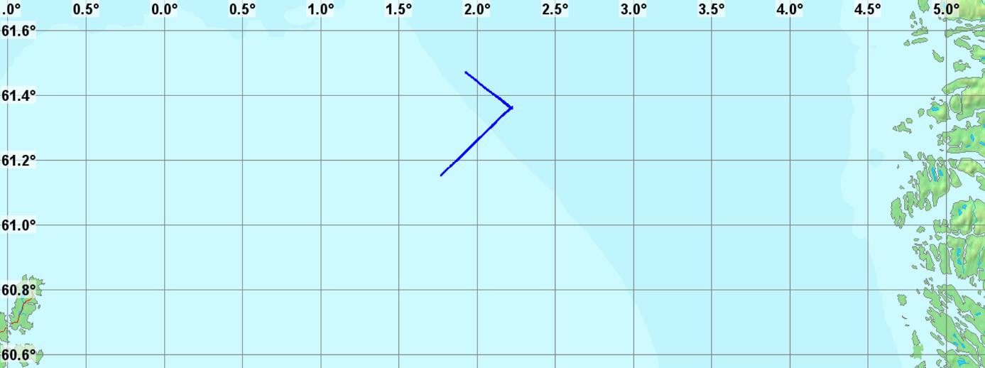
Acoustic data were collected from two transects with the Wassp multibeam sonar (Table 5). The first transect was 18 nm in a southwest direction from the windfarm (SW) and covered the same transect as the gill net stations. The second transect was 10 nm in a northwest direction (NW) (Figure 7). The water depth along the SW transect decreased from 300 m closest to windfarm to 106 m at the furthest point while the NW transect followed the depth contour at about 300 m depth. The acoustic data collection was a secondary priority and adjusted to fit into the gill net sampling times and areas. Fewer data were collected than aimed for due to poor weather conditions. The SW and NW transects were covered twice each. The vessel speed was between 4 and 5 kts during data collection.
The Wassp sonar has a fan of beams arranged perpendicular to the vessel’s alongship axis, and five inspection beams, all operating at 160 kHz. All beam data were stored to computer, but only the inspection beam that pointed vertically down was used in the analyses, as this most closely matches a conventional echosounder. The opening angle of this beam was set to 10 degrees, the sonar ping rate was approximately 1 Hz, and the ping duration was 1 ms. The amplitude response of the sonar was not calibrated.
The Wassp data files were converted to Simrad EK60 format to enable processing in IMR’s acoustic survey software (LSSS). The Korona module in LSSS was used to remove noise from the acoustic data. Acoustic backscatter data were divided into three depth layers; a surface layer at 5 – 25 m, a bottom layer from 25 m above the seabed to 5 m above the seabed, and a mid-layer covering the ranges between the surface and seabed layers. The 25th, 50th and 75th quantiles of volume backscattering strength (Sv, re 1m-1, dB) by ping and within each depth layer (surface, mid and bottom) were calculated. The results are presented as running median values over 11 pings. (~10 s). In addition, a more detailed scrutiny of the data (5 nm steps) was made to identify single targets and aggregations of fish.
Figure 7 . Location of the acoustic transects (blue lines) in relation to the Norwegian coastline to the east and Unst Island to the west.
Table 5 . Overview of the acoustic transects.
Date
Transect
Description
Start Lat (N)
Start Lon (E)
End Lat (N)
End Lon (E)
Start time (UTC)
End time (UTC)
21.03.2023
SW1
Station 8 to 1
61° 18'
1° 83'
61° 36'
2° 21'
04:07
07:43
23.03.2023
SW2
Station 8 to 1
61° 18'
1° 83'
61° 36'
2° 21'
16:09
18:58
23.03.2023
NW1
Station 1 to northwest
61° 36'
2° 21'
61° 47'
1° 93'
18:55
21:54
23.03.2023
NW2
Northwest to station 1
61° 47'
1° 93'
61° 36'
2° 21'
21:54
00:56
3 - Experimental results
3.1 - Gill net catches
3.1.1 - Does species richness vary with distance from the wind farm?
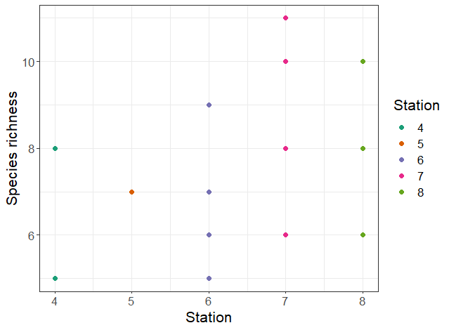
Species richness varied between 5 and 11 species per station. The highest number of species was caught in station 7. There was no statistically significant difference between species richness in the deep and shallow stations (p=0.20). Within the shallow region, there was no relationship between species richness and distance from the set position to the middle turbine (p=0.57) (Figure 8).
Figure 8 . Species richness (number of species present in a catch) per sampling station.
3.1.2 - Does abundance of key species vary with distance from the wind farm?
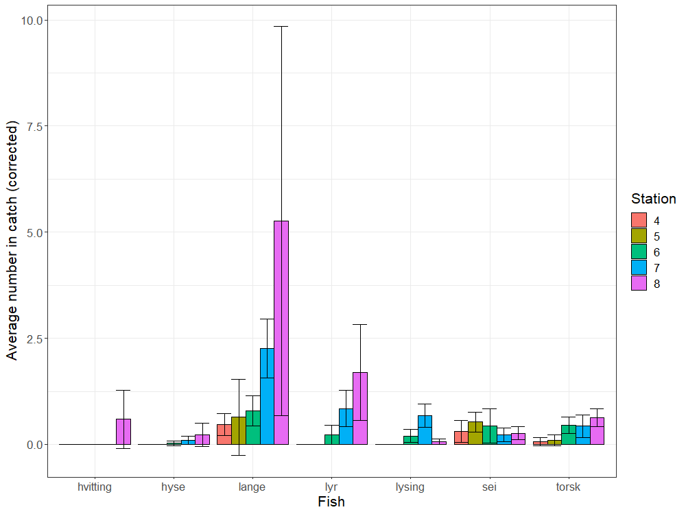
There was some variation in the abundance of the most abundant species in relation to station depth. Whiting, haddock, pollack and hake were only caught in the shallower region, with 0 individuals caught in the deep region (Figure 9). Statistical tests to compare abundances by depth category could therefore not be conducted for these species. As whiting were only caught at station 8, no distance analyses were conducted for this species, either.
Due to having only 3 usable samples from the deep region, the power of statistical tests comparing abundances in the deep and shallow regions was low. Nonetheless, there were significantly higher abundances of cod caught in the shallow than the deep region (p=0.04). However, no significant difference in the abundances of ling could be detected (p=0.38), despite an apparent higher abundance of ling in the shallow catches (Figure 9). There was also no relationship between saithe abundance and depth category (p=0.28).
In the shallow region, there was no relationship between cod, saithe, haddock or hake abundance and distance between set position and the middle turbine (cod: p=0.13; saithe: p=0.45; haddock: p=0.10; hake: p=0.41). There was a significant increase in ling and pollock abundance with increasing distance from the turbine in the shallow region (ling: p=0.04; pollock: p=0.02).
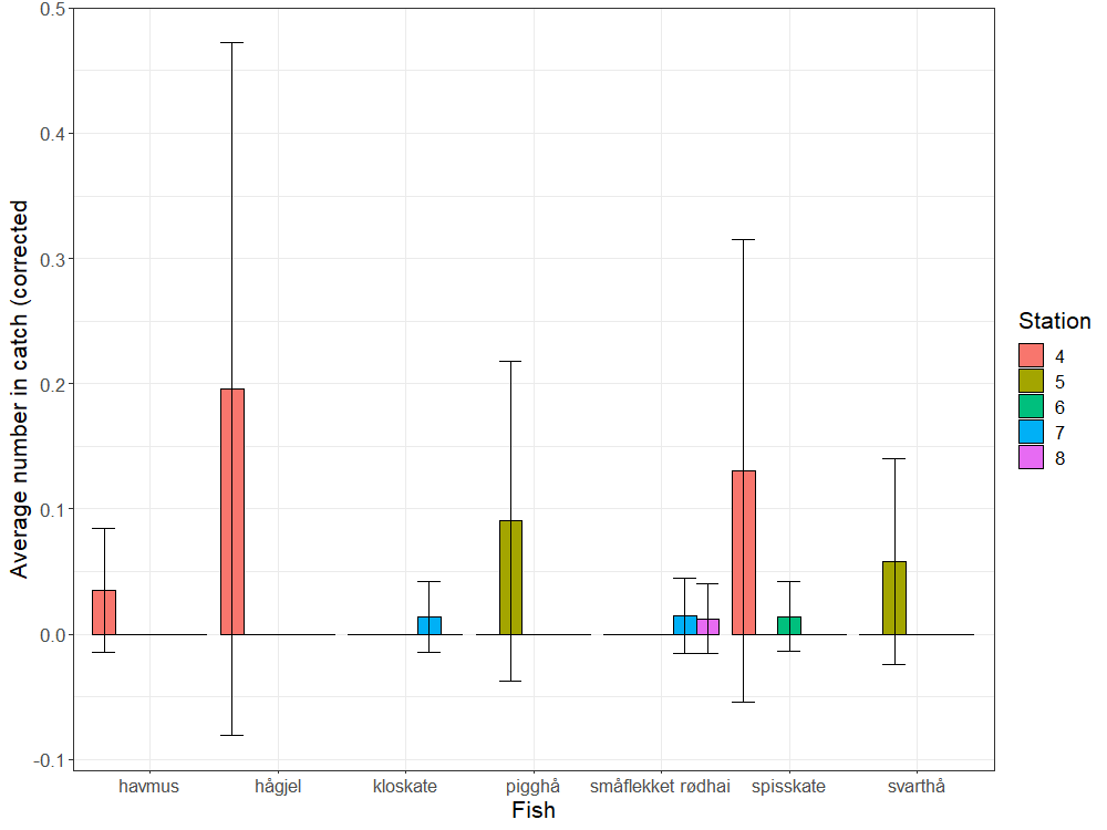
For elasmobranchs, there were too low numbers caught to statistically assess differences. Main species caught were hågjel / blackmouth catshark (Galeus melastomus) and spisskate / longnose skate (Dipturus oxyrinchus) followed by pigghå / spiny dogfish (Squalus acanthias) and svarthå /velvet belly lanternshark (Etmopterus spinax) (Figure 10). Elasmobranchs were mainly caught in the deeper areas, except for kloskate / thorny skate (Amblyraja radiata) and småflekket rødhai / small-spotted catshark (Scyliorhinus canicular) that were only caught in the shallow areas.
Figure 9 . Average number of the most abundant fish caught in gillnets per hour of soak time at the five stations fished during the survey (see Figure 6 ). The catch from Serial 57910 (station 5) was multiplied by three prior to averaging, as 2/3 of the link were completely twisted and unusable, resulting in a representative catch from 1/3 of the link. Standard deviations are shown by error bars.
Figure 10 . Average number of the elasmobranch species caught in gillnets per hour of soak time at the five stations fished during the survey (see Figure 6 ). The catch from Serial 57910 (station 5) was multiplied by three prior to averaging, as 2/3 of the link were completely twisted and unusable, resulting in a representative catch from 1/3 of the link. Standard deviations are shown by error bars.
3.1.3 - Does maturity of key species vary between stations?
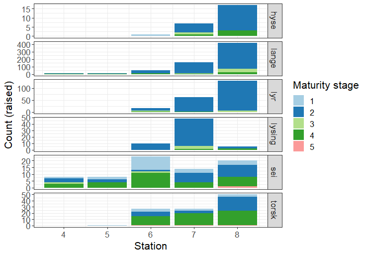
Few spawning fish were caught during the survey (Figure 11,Table 6). Most haddock, ling pollack and hake caught were in the preparation stage. Most saithe and cod caught were spent. During the survey, we caught zero spawning cod, two spawning saithe (one in the deep region, one in the shallow region), one spawning haddock (shallow region), five spawning hake (shallow region) and 10 spawning pollack (shallow region). Relatively many spawning ling were estimated in the catch, with 56 spawning ling in the shallow region, and 0 in the deep region. Due to the low sample sizes, statistical comparisons of proportion of spawning individuals per region or distance were not conducted.
Figure 11 . The distribution of maturity stages by species and station. Note the different y-axes per species. Maturity stages were recorded for the first 20 fish of each species in the catch. In catches with more than 20 individuals of a given species, maturity stages were raised to the total number in the catch. Maturity stages: 1=immature; 2=preparing; 3=spawning; 4=spent; 5=unsure if 1 or 4.
Table 6 . Number of spawning individuals (1) and non-spawning individuals (0) in the survey catches in the deep (stations 4-5) and shallow (stations 6-8) regions.
Species
Spawning
Depth category
Number of individuals (raised)
Haddock/hyse
0
deep
0
1
deep
0
0
shallow
24
1
shallow
1
Ling /lange
0
deep
21
1
deep
0
0
shallow
568.75
1
shallow
57.5
Pollock/ lyr
0
deep
0
1
deep
0
0
shallow
199
1
shallow
10
Hake/ lysing
0
deep
0
1
deep
0
0
shallow
58
1
shallow
5
Saithe/ sei
0
deep
15
0
shallow
56
1
deep
1
1
shallow
1
Cod/ torsk
0
deep
1
1
deep
0
0
shallow
104
1
shallow
0
3.1.4 - Size and condition of common fish
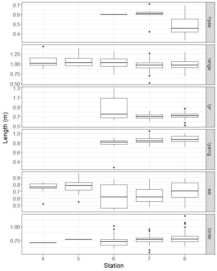
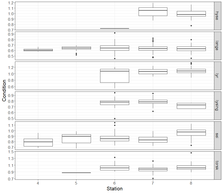
As no whiting, haddock, pollack and hake were caught in the deep region, and as only one usable length measurement for cod in the deep region was available, statistical tests to compare size and condition by depth category could not be conducted for these species. For ling, there was no significant difference between the length or condition of fish caught in the deep and shallow regions (ling length: p=0.07, ling condition: p=0.50) (Figure 12; Figure 13; Figure 14). Saithe were significantly smaller (-0.10 ± 0.04 m, p=0.02) in the shallow region compared to the deep region, and condition factor of saithe was significantly higher (0.07 ± 0.03, p=0.04) in the shallow compared to the deep region.
Within the shallow region, there was a negative relationship between distance to the wind farm and haddock length (-0.02 ± 0.004 m, p=0.004), but no relationship between distance and condition factor (p=0.79). There was no relationship between ling length or condition and distance from the wind farm (length: p=0.92, condition: p=0.11). There was a significant, positive relationship between hake length and distance to the wind farm (0.01 ± 0.004 m, p=0.02), but no relationship between hake condition and distance to the wind farm (p=0.86). Saithe length and condition increased with increasing distance to the wind farm (length: 0.007 ± 0.003 m, p=0.03, condition: 0.006 ± 0.002, p=0.009). Cod length increased with distance to the wind farm (0.004 ± 0.002 m, p=0.01), but there was no relationship between condition and distance from the set location to the middle turbine (p=0.37). Pollock length decreased and condition increased with distance to the turbines (length: -0.004 ± 0.002, p=0.02, condition: 0.006 ± 0.002, p=0.005).
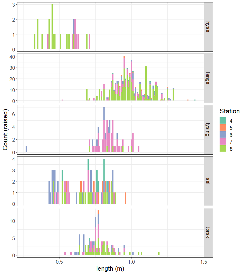
Figure 12 . Length frequency distribution of fish, raised from the measured subsample to the total number caught per catch.
Figure 13 . Length of fish in the measured subsamples, by species and station.
Figure 14 . Condition factor of fish in the measured subsamples, by species and station.
3.1.5 - Stomach content analysis
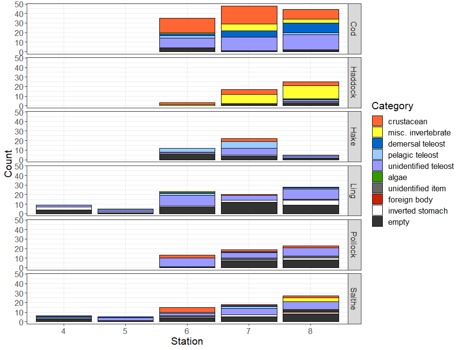
A variety of prey species were identified in the stomach samples (Table 7). Out of the 185 stomach samples, 92 were empty and 23 were inverted. The main prey species were teleost species, while the haddock and cod stomachs also contained crustaceans and invertebrates (Figure 15). The degree of prey digestion ranged from 3 to 5 (IMR system), which made it difficult to categorize prey items to species level.
Figure 15 . Count of all items found in stomachs of sampled fish. The number of inverted stomachs and empty stomachs found within stomach samples are also shown. For breakdown of categories, see Table 7 .
Table 7 . Breakdown of the items within each stomach content category, as shown in Figure 14 .
Stomach category
Prey item
Count
crustacean
Brachyura
12
Caridea
7
Crustacea
15
Euphausiidae
4
Hyas
5
Isopoda
2
Lebbeus
1
Lithodes maja
2
Munida
6
Natantia
7
Paguridae
4
Pandalus borealis
3
Sabinea
6
misc. invertebrate
Actiniaria
1
Aphrodita aculeata
7
Bivalvia
2
Cephalopoda
1
Echinidae
5
Echinus
6
Gastropoda
9
Octopoda
1
Ophiuroidea
6
Polychaeta
4
demersal teleost
Acanthuridae
1
Gadidae
3
Gadus
2
Hippoglossoides platessoides
1
Melanogrammus aeglefinus
1
Pleuronectidae
14
Sebastes
2
Triglops
2
pelagic teleost
Clupea harengus
18
Micromesistius poutassou
1
Pollachius virens
1
Scomber scombrus
4
unidentified teleost
Teleostei
129
algae
Fucales
1
unidentified item
Indeterminatus
10
foreign body
fremmedlegeme
1
inverted stomach
inverted stomach
23
empty
Empty stomach
92
3.2 - Acoustic data
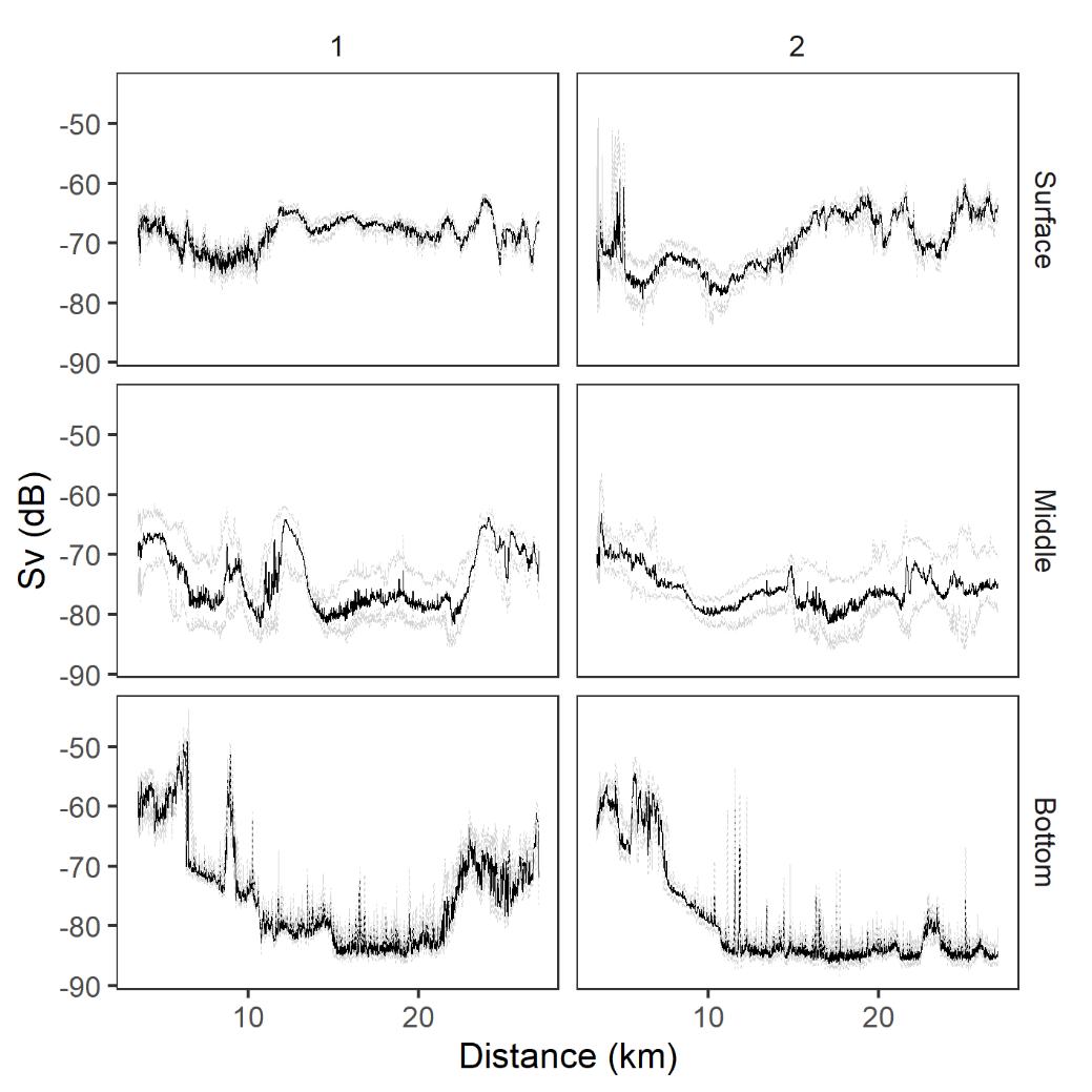
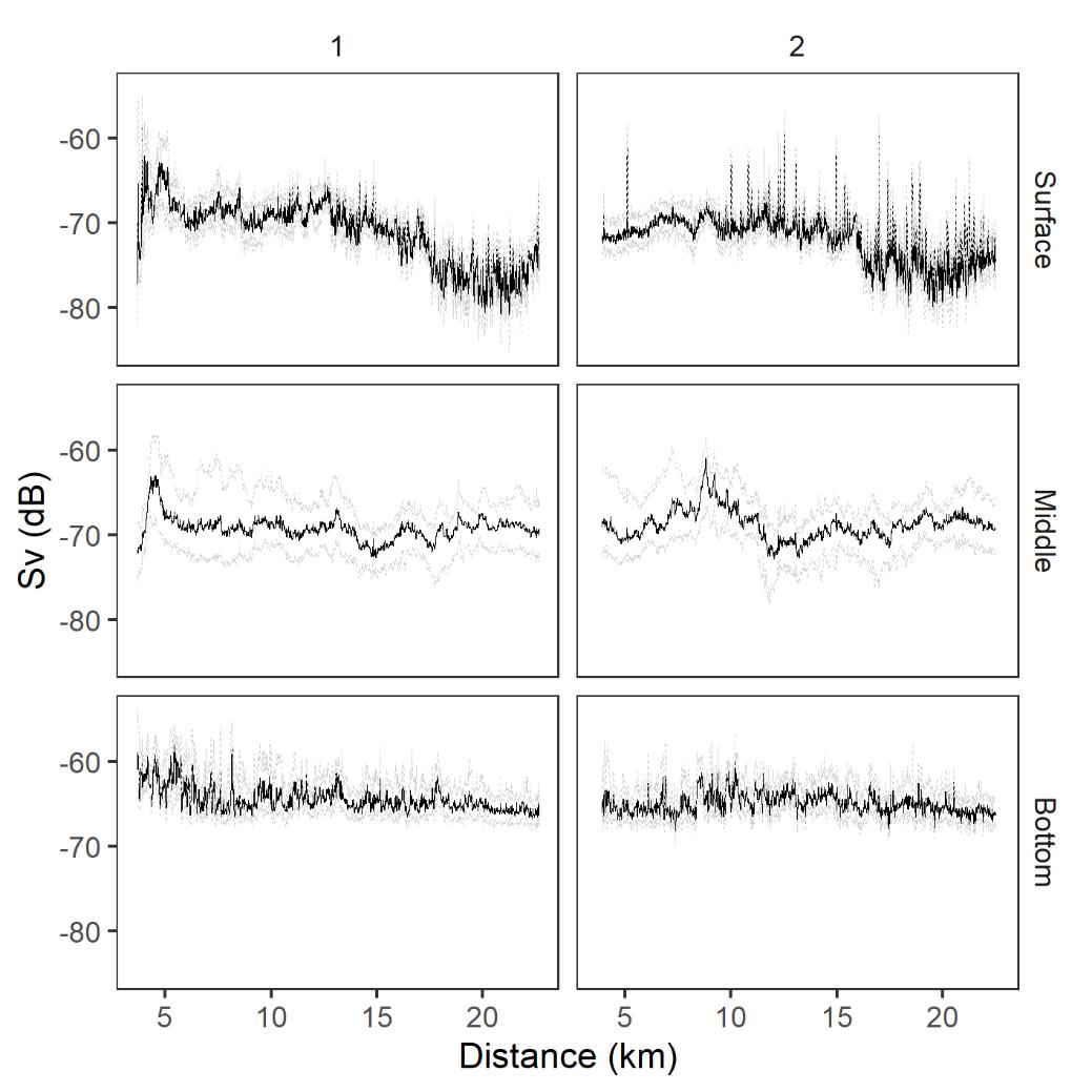
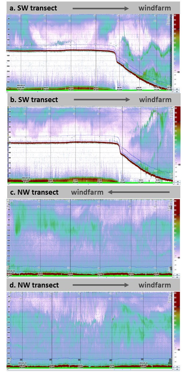
No clear trends in acoustic backscatter strength with distance to wind farm were registered, but these data have not been statistically tested yet (Figure 16; Figure 17). No fish schools were detected in the data, but layers of weak scatterers (plankton or mesopelagic fish) and some individual fish or small groups of fish were registered. The first Southwestern transects was in the early morning between 4 and 7 am starting in the shallow area furthest away from the windfarm (Figure 18a). The second Southwestern transect was in daylight early evening between 4 and 7 pm also starting furthest away from the windfarm (Figure 18b). A weak scattering layer was present in the shallow area distributed from close to surface to 70 m depth and slightly deeper before sunrise. In the deeper water closer to the windfarm a more dense and more concentrated scattering layer was present deeper down.
The NW transects were conducted early evening and, in the night (Figure 18c and d). The first transect started in station one and moved 10 nm in NW direction away from the wind farm. The second transect started 10 nm NW of the wind farm and ended at station one. A scattering layer was present from close to surface and down to 100 m at the start of the transect at 7 pm and moving down to 90 – 200 m 10 pm. There appears to be a slight tendency toward higher density in the area closer to the wind farm based on visual inspection of the echograms (Figure 18).
Figure 16. Acoustic backscatter registered in the Southwestern (SW) transect. Data are presented as median volume backscattering (Sv in dB) values (11 ping running median) in the surface, middle and bottom layers. Distance to windfarm is in the x-axis. Columns 1 and 2 represent the two replicate transects. Dashed light grey lines are the 25th and 75th quantiles.
Figure 17. Acoustic backscatter registered in the Northwestern (NW) transect. Data are presented as median volume backscattering (Sv in dB) values (11 ping running median) in the surface, middle and bottom layers. Distance to windfarm is in the x-axis. Columns 1 and 2 represent the two replicate transects. Dashed light grey lines are the 25th and 75th quantiles.
Figure 18 . Echograms of the four acoustic transects. Backscatter from the centre beam of the wassp sonar 160 kHz. Colour scale indicates strength of backscatter in dB (lower threshold is -82 dB).
4 - Discussion
The most abundant species caught during this survey, which are also of commercial interest, were ling, hake, saithe, cod, pollock and whiting. We found no significant trend in species richness with distance to the wind farm site, but we found some patterns in fish abundance. Hake, haddock, whiting and pollock were only caught in the shallow region further from the wind farm, while catches of cod were significantly higher in the shallow compared to the deeper areas. We were unable to detect statistical difference in abundances of saithe or ling in relation to bottom depth. Maturity of these species did not vary with depth or distance to the wind farm site, except for ling, which showed a higher proportion of mature fish in the shallower areas.
Depth patterns in abundance observed in this survey differed somewhat to the results from the 2022 survey. In 2022, more hake were caught in the deep region compared to the shallow region, while in this survey, hake were only caught in the shallow region. In 2022, higher abundances of ling were caught in the shallow compared to the deep regions, and higher abundances of saithe were caught in the deep regions than the shallow. However, in this survey, no difference in abundance of ling or saithe was detected between depth categories, although the direction of the effects were similar. The depth patterns in cod and whiting abundances were similar between the two surveys. Due to the small sample size for the deep region in this survey, the power of the statistical tests for differences in depth is lower than is 2022, which could have caused the absence of significant effects for ling and saithe.
Trends in fish abundance in relation to distance to the wind farm within the shallow region were similar to the baseline survey in 2022. In both the 2022 and 2023 survey, abundance of ling increased with increasing distances to the wind farm. The distribution of whiting abundance was also similar between years, with whiting mostly (2022) or exclusively (2023) caught at station 8, furthest from the wind farm site. In both surveys, no trends in abundances of cod, saithe or hake were observed with distance to the wind farm in the shallow region. In 2023, pollock abundance increased with distance while no change was registered in haddock abundance. These species were not investigated in the 2022 survey due to low sample sizes (de Jong et al., 2023).
There were some variations in length and condition factor in relation to depth and distance to the wind farm, for some species. Ling and saithe were the only species with large enough sample sizes for statistical comparisons between shallow and deep regions. There was no difference in ling size or condition, while saithe were larger and had lower condition in the deeper region compared to the shallow areas. In 2022, saithe, cod and ling were significantly larger in the deep compared to shallow regions, while hake was smaller in the deep. Within the shallow areas, saithe and hake size and condition and cod size increased, while haddock size decreased with distance to wind farm. In 2022, cod condition increased with distance to wind farm, but no other significant changes were observed.
The gillnets used in the experiments targeted demersal species, but the stomach content analyses can reveal information about pelagic species in the area too. In 2022, pelagic fish were registered in most of the stomachs that were analysed. This year, fewer pelagic species were identified, mainly herring and some mackerel in the hake stomachs. However, a substantial proportion of the items were allocated to unidentified teleosts. The degree of digestion was too high for a more detailed identification. The stable isotope analysis of the muscle samples taken during this survey can reveal additional information about the diets of sampled fish. These have not yet been analysed but should be prioritized.
The acoustic data collection was a secondary objective on this survey and was adjusted to fit in between the fishing trials and the instrumentation available on the vessel. Data were collected both at day and nighttime. However, with only two replicate transect coverages it is unlikely that changes related to the presence of the windfarm can be detected. Pelagic species vary in presence, density, and vertical distribution due to daily vertical migration behaviours, but also due to random factors. Pelagic fish are highly mobile, and the area would need to be covered far more extensively in time and space to get a good overview. No schools were detected in the data, but layers of weak scatterers were present. These were not registered in the 2022 survey. With only one acoustic frequency, a system that was not calibrated and without ground truthing the acoustic data it will not be possible to allocate the acoustic registrations to species. However, changes in the patterns in backscatter after establishment of the wind farm would reflect changes in marine organisms, it will thus be interesting to monitor the acoustic backscatter levels and trends during the operational phases to see whether these change or remain the same. In 2023, GO Sars (Utne Palm et al., 2023) covered the area far more extensively compared to the acoustic data collected in this cruise.
Fish capture studies provide detailed information about target species abundance, distribution, and biology (size, condition, maturity, and diet). The sampling method can be considered wasteful, but in this study, catches were kept on board and sold at the end of the survey with no need to discard samples. Unfortunately, poor weather conditions prevented us from sampling stations 2, 3 and 4. Attaching nets in the soft bottom in the slope proved to be challenging. In the shallow area where the seabed was even no such problems were experienced. Drifting was also experienced in the 2022 experiment at one of the stations (6), this station was therefore moved. Since currents in this area are stronger with full moon, future cruises should avoid that in the planning. In addition, this method should be combined with more dedicated acoustic surveys. There is also a need to improve the gillnet sampling design to be less vulnerable to currents and bottom conditions, maybe by using heavier weights.
This and the survey in 2022 (de Jong et al., 2023) have collected highly valuable and unique information at a high spatial resolution about demersal fish species before and in an early operational stage of the Hywind Tampen offshore wind power field. We expect that the distance-based sampling method will allow us to detect fine scale temporal and spatial changes that the wind may cause. However, additional sampling is required to monitor the development of the fish community over time.
5 - Acknowledgements
The cruise was financed by the Norwegian Ministry of Trade, Industry and Fisheries. We thank the captain and crew on Nesejenta for their good cooperation. We also thank Equinor for sharing information and cooperation during the cruise.
6 - References
Anne Christine Utne Palm, Henrik Søiland, Anne Kari Sveistrup, Angelika Renner, Rebecca Ross, Frithjof Moy, Mostafa Bakhoday Paskyabi, Atle Totland, Sigurd Hannaas, Karen de Jong, Genoveva Gonzalez-Mirelis, Terje Hovland, Geir Pedersen, Jan Frode Wilhelmsen, Markus Antti Majaneva, Sverre Waardal Heum, William Skjold, Stig Vågenes, Georg Skaret, Finn Corus, Andrey Voronkov, Patrick Vågenes and Leonard Kielland. 2023. Cruise report Hywind Tampen 13 to 28 March 2023 — Cruise no. 2023001004 G.O. Sars. Report series: Toktrapport 2023-10 ISSN: 1503-6294 Published: 24.08.2023. https://www.hi.no/en/hi/nettrapporter/rapport-fra-havforskningen-en-2023-32
Karen de Jong, Kate McQueen, Nils Roar Hareide, Maria Tenningen ,Gavin John Macaulay, Markus A. Majaneva Research. 2023. Fisheries survey in the offshore wind power field Hywind Tampen before development. Rapportserie: Toktrapport 2022-15 ISSN: 1503-6294 Publisert: 09.01.2023 Oppdatert: 20.02.2023. https://www.hi.no/hi/nettrapporter/toktrapport-en-2022-15
Methratta, E.T., 2021. Distance-Based Sampling Methods for Assessing the Ecological Effects of Offshore Wind Farms: Synthesis and Application to Fisheries Resource Studies. Frontiers in Marine Science 8.