Brisling er en viktig del av økosystemet i mange norske fjorder, der fisk, fugl og sjøpattedyr beiter på den. For å kunne overvåke endringene i brislingbestandene og gi et bærekraftig kvoteråd på brisling, gjennomføres det regelmessige akustiske-tråltokt i fjordene med forskningsskip i regi av HI. Det har blitt stilt spørsmål ved om kvaliteten på dataene som samles inn med disse skipene, da man har indikasjoner på at en del av brislingstimene står for nær overflaten til å kunne måles med skipets ekkolodd. I tillegg er det krevende å navigere nær land og på grunne områder med disse store skipene. Under årets brislingtokt med FF Kristine Bonnevie ble det derfor gjennomført et eksperiment der ekkoloddata (200 kHz) ble samlet inn med Havforskningsinstituttets stillegående kajakkdrone i Årdalsfjorden på kvelden 15. august og dagtid 16. august. Det ble målt omtrent like stor mengde og ganske lik horisontal fordeling av brisling i de to forsøkene. En del stimer ble observert så nært land at de er utilgjengelig for et stort skip. Forsøket viste at brislingen stod svært nær overflaten på kveldstid; 63% av den akustiske tettheten stod i de øverste 8 meterne, som er dypet som regnes som skipets blindsone. På dagtid sto 24% av brislingen i denne blindsonen. Forsøket viser at man bør videreutvikle teknologi som kan måle fisk som står nær overflaten for å kunne overvåke brisling, og at fremtidens tokt bør inkludere denne type teknologi. Det vil imidlertid fremdeles være behov for et fartøy som kan tråle etter biologiske prøver.
Measuring distribution and density of sprat in Årdalsfjorden with a kayak drone
— 15-16 August 2020
Report series:
Rapport fra havforskningen 2020-28
ISSN: 1893-4536
Published: 09.09.2020
Project No.: 14558 Kystbrisling (internal project), Acoustic kayak drone (RCN Project number 243941), CoastRisk (RCN Project number 299554)
Research group(s):
Acoustics and Observation Methodologies
,
Pelagic fish
Subject:
Sprat
Program:
Coastal Ecosystems
Research group leader(s):
Rolf Korneliussen (Acoustics and Observation Methodologies)
Approved by:
Research Director(s):
Geir Huse
Program leader(s):
Jan Atle Knutsen
Norsk sammendrag
Summary
Sprat is a key species in several Norwegian fjords, as an important prey for fish, sea mammals and sea birds. The sprat populations are monitored with routine acoustic-trawl surveys using a large research vessel, which provide the main scientific basis for sprat quota advices. Previous survey observations indicate that a significant fraction of the sprat population can be found close to the sea surface and thereby in the acoustic blind zone of the echosounder mounted below the vessel. In addition, fish may avoid the approaching vessel, and thereby measure less acoustic density. Furthermore, a large research vessel cannot operate in shallow waters and is difficult to maneuver close to the shore. In an experiment carried out in Årdalsfjorden in the evening 15 August and during daytime 16 August, the distribution of sprat was measured with a kayak drone installed with a 200 kHz echosounder. The geographical distribution and the mean acoustic density were similar between the two coverages. The experiment showed that 63% of the fish density was observed closer to the surface than 8 meters, which is the acoustic blind zone of research vessel. At daytime, the fish was distributed deeper, but 24% of the fish was still distributed closer to the surface than 8 m. This experiment show that future sprat surveys should be carried with silent vehicles where the echo sounders are mounted near the surface. A larger vessel is though also needed for trawling for biological samples.
1 - Introduction
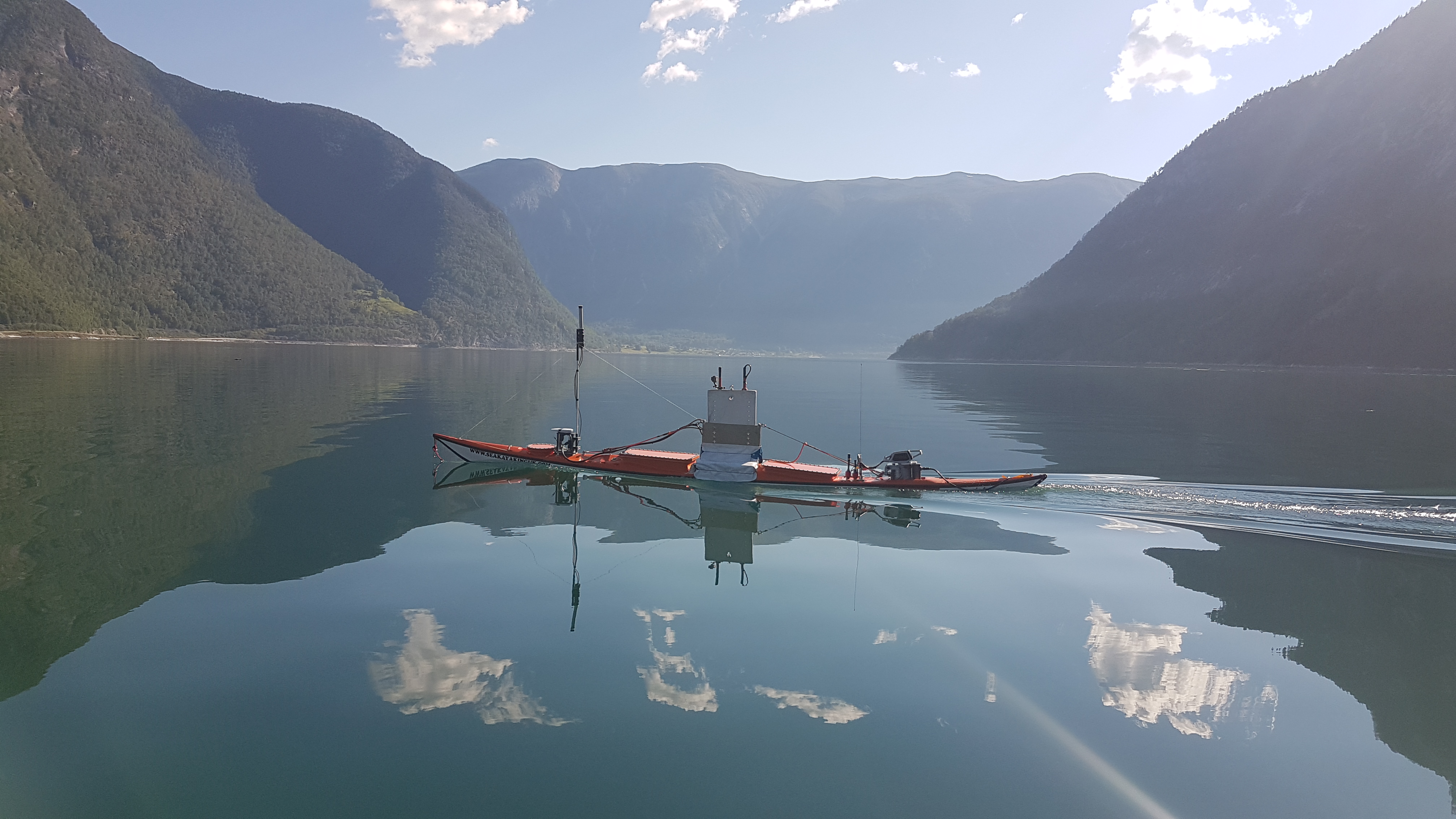
Droneferd i Sognefjorden. Photo: Espen Johnsen
Årdalsfjorden is a fjord arm situated in the inner part of Sognefjorden, the deepest fjord in Norway (1303 m) and the second longest fjord in the world (205 km). In this ecosystem, the small clupeid sprat ( Sprattus sprattus L.) is a key species. It feeds on zooplankton (Falkenhaug and Dalpadado 2014) and is itself an important prey for both larger fish, sea mammals and birds (Bakketeig et al. 2017) thus linking the energy from zooplankton to larger animals. In the beginning of the 19 th century, the sprat fishery delivered quite large amounts of sprat to canning factories along the coast of southern Norway, producing canned “sardines” in oil (NOU 1979). After the 1970ies, the catches have been much lower, but also the fishing effort (Bakketeig et al. 2017). Surveying sprat in the Norwegian fjords is important due to the role of sprat in the ecosystem. In fjords with a fishery for sprat, like Sognefjorden, surveys are also needed to give adequate advice for the managers setting quota limits.
The sprat and herring populations in the Norwegian fjords are traditionally monitored using acoustic-trawl surveys carried out by a large research vessel (Kvamme et al. 2010), where the echosounders are mounted on a retractable keel. As standard, the keel is not extended during the fjord cruises and the transducer depth is therefore around 6 m. Assuming a near field of about 2 m (SIMRAD 2015) for a 38 kHz echosounder, this makes a total acoustic blind zone of about 8 m. In addition, several studies show that the fish avoid the approaching vessel, and thereby measure less acoustic density than the “undisturbed” true density of fish near the surface (De Robertis and Handegard 2013 ). Furthermore, a large research vessel cannot operate in shallow waters and is difficult to maneuver very close to the shore.
To examine the challenges described above, an initial list of main objectives and associated methods was set up for the kayak drone experiments. These were:
Measure the abundance of sprat in one or more side fjords to the Sognefjord using the kayak drone during day and night.
Investigate if sprat is distributed close to the shore and/or in shallow waters not navigable for the large research vessel RV Kristine Bonnevie.
Investigate if sprat is distributed in the surface blind zone of RV Kristine Bonnevie.
Investigate if sprat avoids RV Kristine Bonnevie.
2 - Methods
2.1 - Planning of the surveys
Årdalsfjorden was chosen as the experimental site as a survey coverage with RV Kristine Bonnevie showed schools of sprat in this side fjord. As one of the objectives was to observe the sprat distribution very close to the shore, we needed accurate map data to generate an accurate stratum polygon and cruise transects. We have access to high resolution map data from Kartverket (https://www.kartverket.no/)., and the following procedure was used to generate a stratum and survey transects for the evening/night (run 1) and daytime (run 2) coverages of the fjord (Figure 1):
The high-resolution map was loaded into the map program OpenCPN (https://opencpn.org/).
In OpenCPN, a closed route (GPX format) was made interactively for Årdalsfjorden, with the outer boundaries 30 meter from the shore.
An R script was made to convert the GPX route to a WKT polygon stratum file which is used by the surveyPlanner function in the R-package Rstox 1.11.1 (https://www.hi.no/hi/forskning/prosjekter/stox).
For the run 1 and run 2 experiments, the Rstox::surveyPlanner was used to generate evenly distributed transects with random start position in a zig-zag pattern across the fjord, using the following settings in surveyPlanner:
Run1: surveyPlanner(projectName=out.wkt, plot=FALSE, type="EqSpZZ", knots=5, hours=4,bearing="along",retour=FALSE,reset=T, seed=100,rev=TRUE))
Run2: surveyPlanner(projectName=out.wkt, plot=FALSE, type="EqSpZZ", knots=5, hours=4,bearing="along",retour=FALSE,reset=T, seed=777,rev=TRUE)
The tracks were converted in R to GPX-format and imported into OpenCPN, where we converted the tracks to routes.
The Route files were copied to the kayak drone computer with waypoints. These routes govern sailing of the drone in autonomous mode as used here.
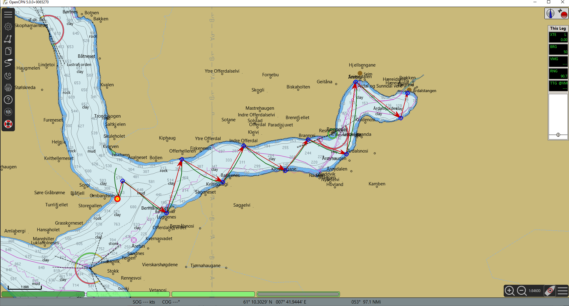
The complete sailed distance for each of the two coverages was approx. 16 nmi and the drone speed was set to 5 knots (50 % engine power). In run1 the battery for the propulsion motor ran out of power at the final transect (1 nmi from the end), while run 2 was completed as planned.
Both surveys were successfully carried out.
One of the man-over-board (MOB) boats of RV Kristine Bonnevie was equipped with an antenna and a computer for remote access to the drone via a Wi-Fi link. This equipment was powered by a small 12V DC lead battery. The MOB boat acted as the control centre during the surveys.
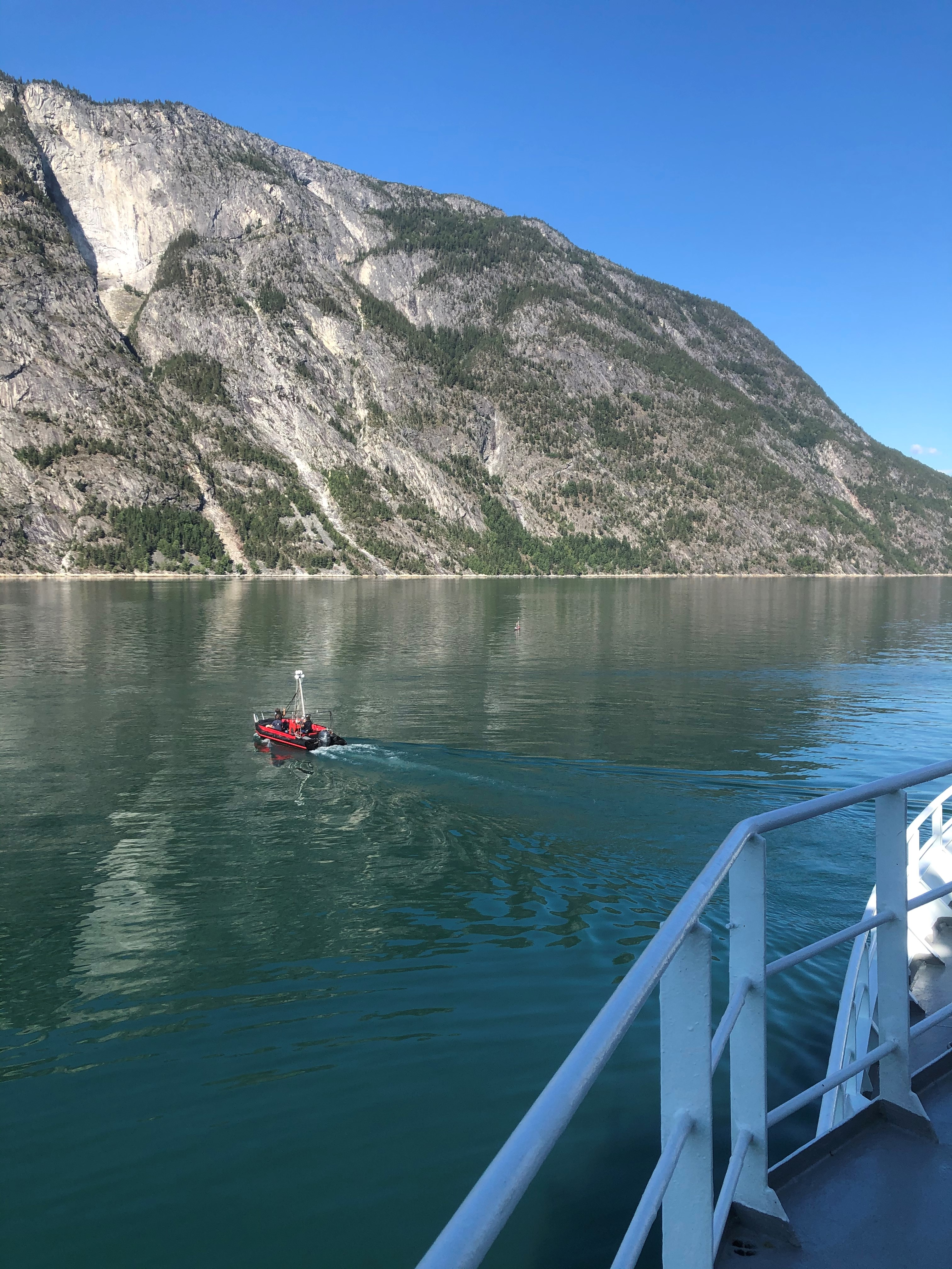
The MOB boat (Figure 2) was used as a control centre since the experiments were conducted in a fjord trafficked by leisure boats. This was a safety measure and allowed for a quick intervention if needed. No intervention of the kayak drone operation was needed.
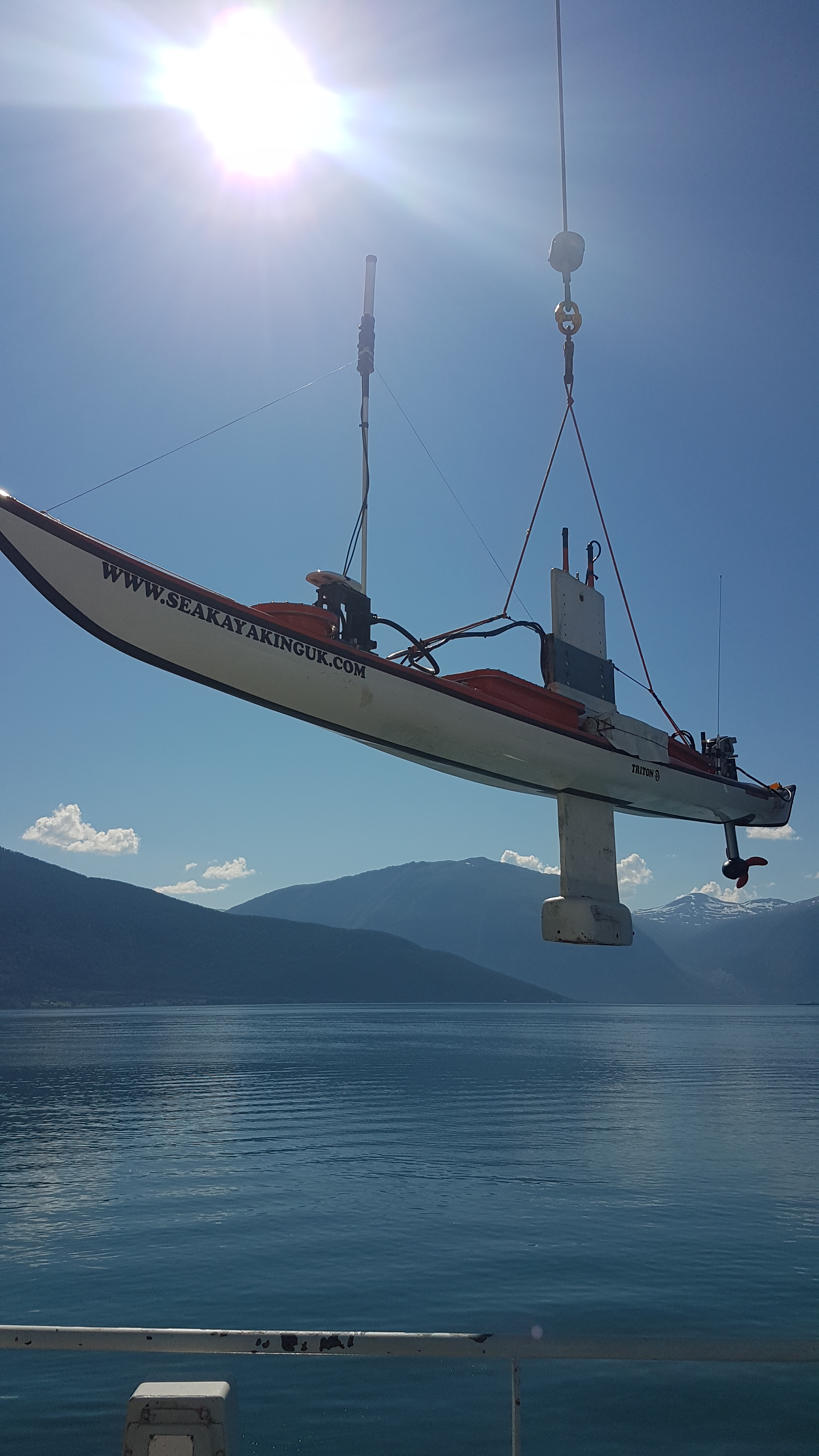
2.2 - Description of the kayak drone
The kayak drone is an autonomous unmanned surface vehicle built on a modified 7-meter-long Nigel Dennis Triton double kayak ( https://www.seakayakinguk.com/ ). Propulsion is given by a Torqeedo 2 HP electric outboard motor ( https://www.torqeedo.com/en). The kayak drone has a maximum speed of 8 knots. The motor has a large propeller and low revolutions per minute (RPM), giving a very silent travel through the water. Operation time of the Torqeedo motor with a travel speed of about 5 knots is about 4 hours with the current battery. The kayak hull has free space for a second battery which will double the sailing capacity. On the current version, a SIMRAD EK60 200 kHz echo sounder is mounted, but there is space for a second echo sounder. The transducers are mounted in the bulb at the end of a 1.5 m retractable centerboard (keel) (Figure 4). This keel brings the transducer below the surface bubble layer and provides stability to the kayak drone.
The central control unit and data logger is a ruggedized Window 10 computer. The computer also contains EK60 echo sounder software, and it receives data from the installed GPS vector compass that output accurate position, UTC time, heading, speed over ground, tilt, roll and rotation speed. An AIS transceiver is also integrated in the system to increase the visibility of the kayak drone to other vessels.
A marine Wi-Fi link between the drone and mother-vessel, and the use of remote control VNC software, makes it possible to access the kayak drone computer from an external computer from a distance. The kayak drone computer screen is shown remotely, and keyboard and mouse actions are transmitted to the drone. The drone may be operated without remote access if preferred.
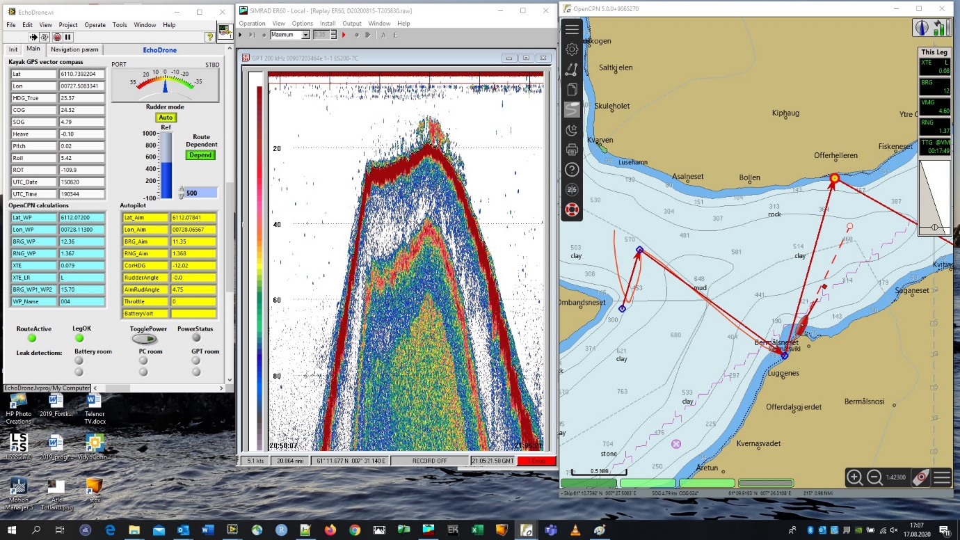
The generic computer solution enables future implementation of new sensors and software in the drone without major changes to the overall system. The sailing and autonomous operation of the drone is governed by the joint effort of an open source chart program, OpenCPN ( https://opencpn.org/ ) and a system made Labview ( https://www.ni.com/en-no/shop/labview.html ) control software (EchoDrone.exe). The two programs process and exchange data. EchoDrone.exe is responsible for sending throttle commands to the propulsion engine and rudder command to the rudder stepper motor.
In standard mode, the user set up a route with waypoints for the desired sailing in the chart of OpenCPN. The drone will then follow the route to the end and stop. OpenCPN uses well tested algorithms for navigation and output processed data for the use of the EchoDrone.exe control software. Kartverket ( https://www.kartverket.no/ ) has provided access to high resolution and accurate chart data that are uploaded into OpenCPN.
2.3 - Scrutinizing echo sounder data (LSSS)
Data were recorded with a Simrad EK60 200kHz echo sounder where the transducer was mounted in a drop keel 1 m below the sea surface. For the first run data were collected up to 200 m range and with a ping interval of 0.79 seconds. For the second run the ping interval was changed to 0.35 seconds. Due to time constraints the echo sounder was not calibrated. It will be calibrated when it’s back in Bergen.
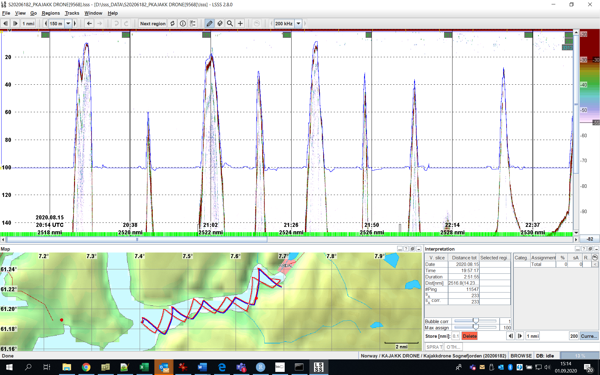
Raw acoustic data were scrutinized in LSSS 2.8.0 software (Korneliussen et al. 2016). All “false bottom” was marked as “schools” without assignment to any acoustic categories. Shadow from the steep walls of the subsea were excluded from the “layer region”, and the “main region” boundaries were set between 2 m and 100 m. By using a 2 m upper boundary, the near field of the transducer is not included, and as no strong targets were observed in deeper waters, we didn’t scrutinize data deeper than 100 m. The only acoustic LSSS category used was “20” = “sprat” (Figure 6). To avoid unwanted weaker targets like plankton to influence the results we used a threshold of -55 dB. The scrutinized data were stored at a resolution of 0.1 nmi horizontal and 1 m vertical and exported in units of Nautical Area Scattering Coefficient (NASC; m 2 nmi -2 ).
2.4 - Data analyses of NASC data
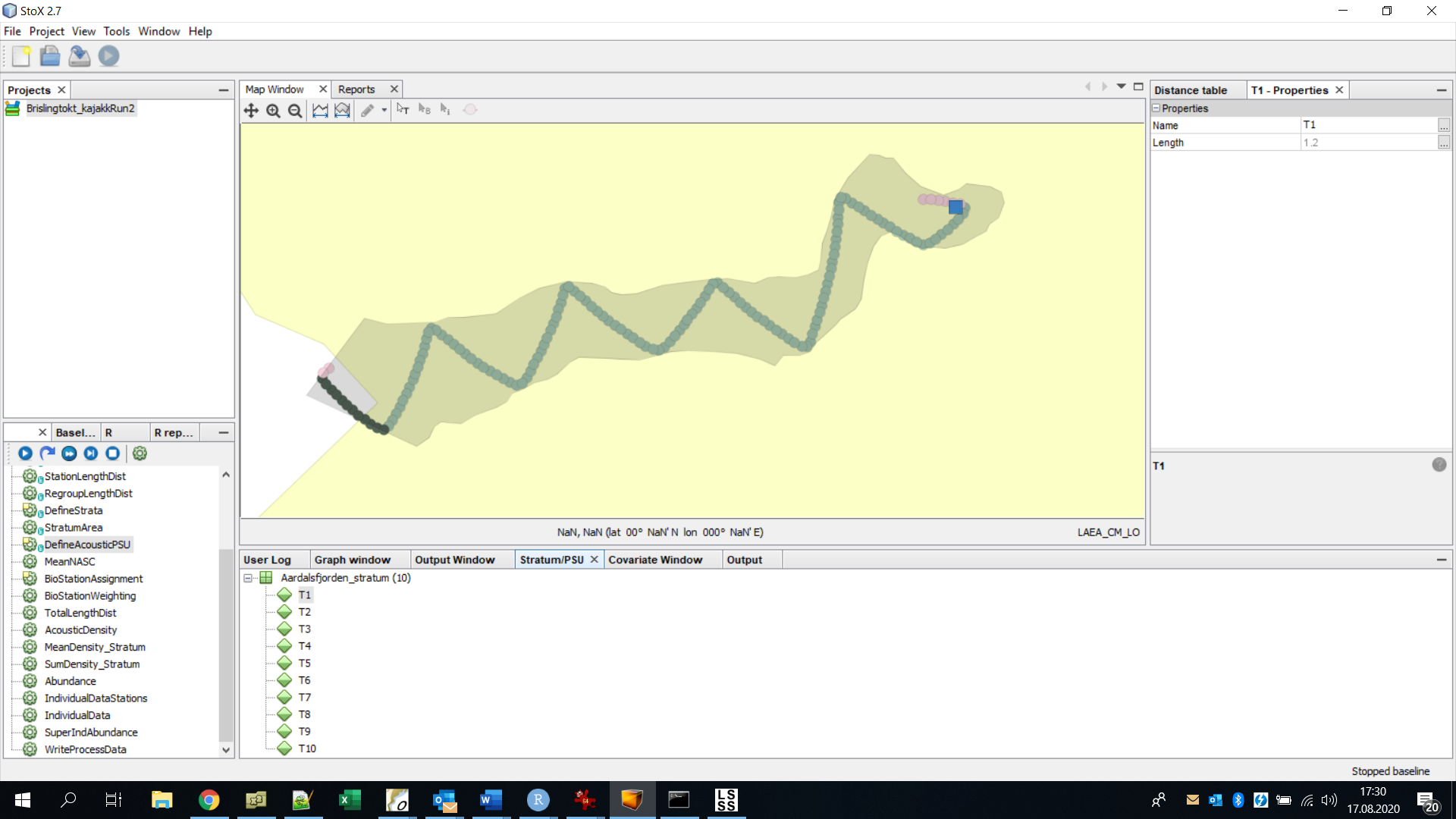
The NMD acoustic.xml files produced by LSSS were imported into StoX 2.7 (Johnsen et al. 2019). StoX projects were created for respectively run1 and run2 (Figure 7), and the acoustic primary sampling units were defined. All analyses were carried out in R (R Core Team 2019) where the R-package Rstox 1.11 (https://www.hi.no/hi/forskning/prosjekter/stox) was used to run the StoX projects and import the data to R.
3 - Summary of the performance of the kayak drone system
The kayak drone performed well, without any major technical problems during this survey.
The remaining main technical issue of the kayak drone is the poor performance of the WiFi link between drone and mother-vessel. The connection breaks down from time to time. However, the drone is autonomous and continues the planned surveying also without this link.
During this survey, some minor needs for improvement were identified and mostly corrected:
The shape of the kayak is sensitive to the athwartship weight balance. During run1, the track of the drone formed a “banana-shaped” curve to the starboard side of the ideal transect line. The balance was adjusted before run2, giving an improved performance. Further adjustment is planned.
A minor leakage (a few centilitres) into the GPT chamber was detected midway during run2. The alarm in the drone gave indications. After the experiment was completed, the leakage was identified to be related to a tube through the deck with poor sealing. This will be fixed after the survey.
If longer operation time is desired, an extra propulsion battery could be installed, doubling the operation time. New types of batteries for the instrumentation may be needed as well. These are less heavy and with higher capacity than the current lead batteries.
During run2 the drone turned for a new transect 50-60 meter to early. This will be corrected by a setting in OpenCPN for the next similar survey.
4 - Preliminary results
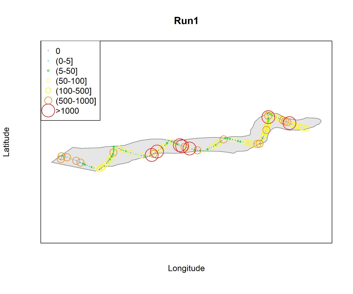
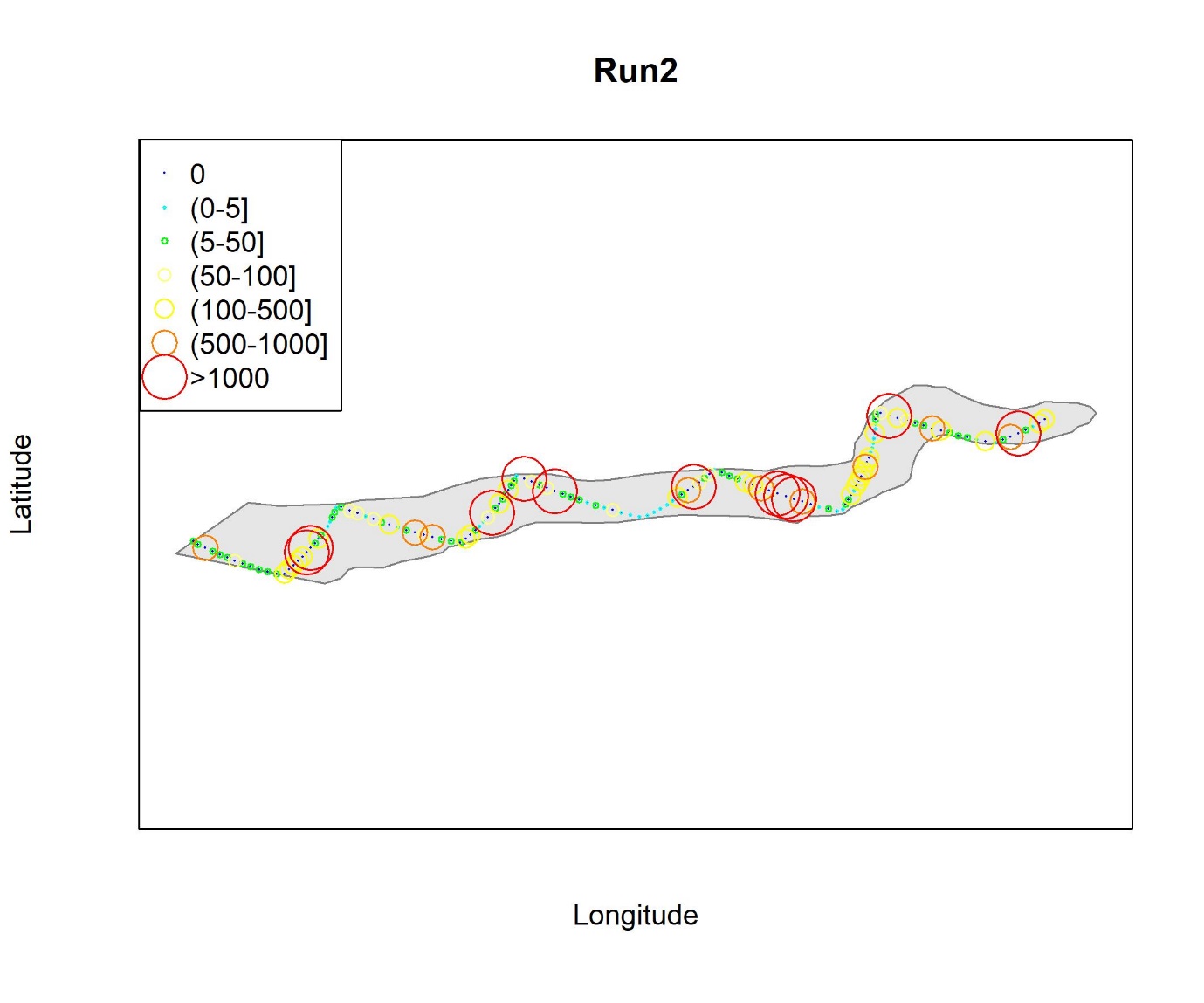
The focus of the experiment was to examine the vertical and geographical distribution of acoustic density of sprat and/or herring in a typical fjord in the Sognefjord area measured with the kayak drone. Figures 8 and 9 show that the density of fish is distributed all over the fjord, and the mean acoustic density was very similar between the two coverages with a mean NASC of 312.5 and 335.6 in run1 and run 2, respectively. The relative sampling error was 27% in run 1 and ~24% in run2 (see Jolly and Hampton 1990 for method). Some areas had more and denser schools, but no clear west-east trend was seen. No clear density structure with distance from shore was evident, however, large densities were observed in areas close to the shore where a large research vessel never operate.
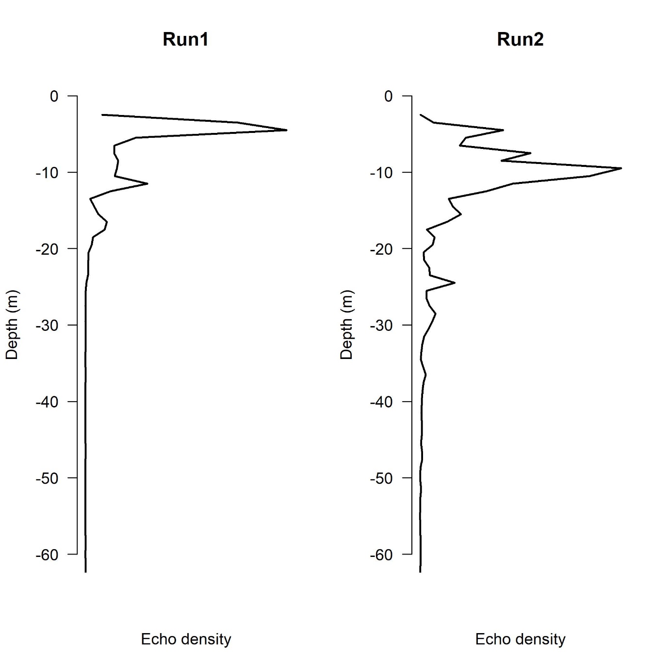
In run1, which was carried out from dusk till almost midnight ( 15/8 UTC 18:20 – 21:31 ), 63% of the fish density was observed closer to the surface than 8 meters, and 89% of the fish was distributed shallower than 15 m (Figure 10). At daytime, (run2, 16/8 UTC 11:34 – 15:52 ) the fish was distributed deeper, and 24% of the fish was distributed closer to the surface than 8 m, and 78% was distributed shallower than 15 m (Figure 10).
In the survey with RV Kristine Bonnevie co-occurring with this experiment, biological samples from acoustic registrations were achieved by targeted trawl hauls with a small pelagic trawl (Harstad) in the registration depth. In trawl catches close to the survey area, from the inner part of the Årdal fjord and the outer part of the Luster fjord, small sprat (Årdal 56%, Luster 98%) and herring (18% in Årdal, <1% in Luster) were dominating in the catches (Table 1).
Table 1. Species composition and length distribution of the catches taken in two trawl stations in the survey area.
5 - Discussion
The kayak drone experiment was successfully carried out. The planned survey tracks were almost completed (except the last 1 n.mi. of the first run), and the acoustic data quality was good. The scrutinizing operation in LSSS used an easy approach as the focus was to categorize one single category of stronger acoustic targets. It is not possible to separate herring and sprat based on the acoustic signal, and other species like sticklebacks may be included in the defined acoustic category “sprat” used in this experiment. However, as the sprat dominated the catches in the Årdal fjord, it is also likely that it dominated the acoustic backscattering observed from the kayak drone. Nevertheless, the acoustic density for “sprat” was distributed relatively evenly over the fjord, and high densities were found in shallow and deeper parts of the fjord. Similar, high densities were observed in the centre of the fjord and near the shore. Thus, the kayak drone shows that “sprat” is distributed in parts of the fjord that are too shallow and to close to the shore to be monitored by a large research vessel. More data analyses and more experiments are needed to quantify the impact of this poor coverage to the historical survey time series.
The mean density of “sprat” was very similar between the two runs, which indicates that kayak drone was able to monitor the true distribution of “sprat” even at night when the fish was distributed closer to the surface. The depth distribution of the acoustic density of “sprat” shows that a large part of the “sprat” density is in the acoustic blind zone of a typical large research vessel (about 8 m; transducer depth + near field of 38 kHz). In run1 (evening and night) only one third of the NASC value was distributed deeper than 8 m, and in run2 (daytime) 70% of the NASC value was distributed deeper than 8 m. Several studies show that a strong vessel avoidance should be expected for clupeids (De Robertis and Handegard 2013), and therefore, it is likely that less than 50% of the sprat density in the fjord could be measured even at daytime.
In summary, the kayak drone surveys show that future sprat surveys should be carried with silent vehicles where the echo sounders are mounted near the surface. A larger vessel is though also needed for trawling for biological samples.
6 - Acknowledgements
We are grateful for the assistance, service and good help from the crew and scientific staff onboard RV Kristine Bonnevie during the experiments. This study was funded by the internal project 14558 Kystbrisling and the RCN project "Kyst – Coast-Risk, Assessing cumulative impacts on the Norwegian coastal ecosystem and its services" (299554). The kayak drone was built under the “Acoustic kayak drone” project, funded by the The Research Council of Norway (project number 243941).
7 - References
Bakketeig, I.E., Hauge, M., Kvamme, C. (red.) (2017). Havforskningsrapporten 2017. Fisken og havet, særnr. 1-2017. https://issuu.com/havforskningsinstituttet/docs/havforskningsrapporten_2017
De Robertis, A., & Handegard, N. O. (2013). Fish avoidance of research vessels and the efficacy of noise-reduced vessels: a review. ICES Journal of Marine Science , 70 (1), 34-45.
Falkenhaug, T., & Dalpadado, T. (2014). Diet composition and food selectivity of sprat ( Sprattus sprattus ) in Hardangerfjord, Norway. Marine Biology Research , 10(3), 203-215. DOI: 10.1080/17451000.2013.810752
Johnsen, E., Totland, A., Skålevik, Å., Holmin, A. J., Dingsør, G. E., Fuglebakk, E., & Handegard, N. O. (2019). StoX: An open source software for marine survey analyses. Methods in Ecology and Evolution , 10 (9), 1523-1528.
Jolly, G. M., & Hampton, I. (1990). A stratified random transect design for acoustic surveys of fish stocks. Canadian Journal of Fisheries and Aquatic Sciences , 47 (7), 1282-1291.
Korneliussen, R. J., Heggelund, Y., Macaulay, G. J., Patel, D., Johnsen, E., & Eliassen, I. K. (2016). Acoustic identification of marine species using a feature library. Methods in Oceanography , 17 , 187-205.
Kvamme, C., Falkenhaug, T., & Dalpadado, P. Toktrapport Epigraph – økosystemtokt Hardangerfjorden, oktober 2010. Brisling og dyreplankton. F/F Håkon Mosby. Tokt nr. 2010-622, 25.–30. oktober 2010. https://www.hi.no/resources/publikasjoner/toktrapporter/2010/130424_toktrapport_2010622.pdf
NOU 1979. Fiskehermetikkindustrien. Sardinsektoren. NOU 1979:12. 41 p.
R Core Team (2019). R: A language and environment for statistical computing. R Foundation for Statistical Computing, Vienna, Austria. URL https://www.R-project.org/.
SIMRAD 2015. Installation manual. Simrad EK60 Scientific echo sounder. https://www.kongsberg.com/globalassets/maritime/simrad/echo-sounders/ek60/installation/164696ab_ek60_installation_manual_english.pdf