Antarctic krill and ecosystem monitoring survey off the South Orkney Islands in 2023
Author(s):
Bjørn Krafft
, Ronald Pedersen
, Guosong Zhang
, Sebastian Menze
, Astrid Fuglseth Rasmussen
, Hege Skaar
(IMR), Julian Dale (University of St. Andrews), Martin Biuw
(IMR), Chris Oosthuisen (University of Cape Town) and Andy Lowther (Norwegian Polar Institute)
Cruise leader(s):
Bjørn Krafft
(IMR)
Miljøovervåking langs 5 faste transekter utenfor Sør-Orknøyene i Sørishavet utføres årlig (siden 2011) av Havforskningsinstituttet. Denne rapporten presenterer forskningsaktivitetene som ble gjennomført iløpet av den Australske sommersesongen 2023, med foreløpige resultater. Data brukes til å beregne biomasse av antarktisk krill (Euphausia superba) samt kartlegge utbredelse og demografisk sammensetning av krill, men også andre makrozooplankton og fisketaxa. Visuelle observasjoner av hval og sel registreres systematisk langs transektene mens det er dagslys. Et pilotstudie for å overvåke hvalens body-condition ved å bruke dronefotografier ble gjennomført, samt et satellitt-telemetristudie på pingviner for å beregne energiske behov i hekketiden samt potensiell beite-overlapp med krillfiskeaktiviteter.
Summary
Environmental monitoring along 5 set transect lines off South Orkney Islands in the Southern Ocean have been carried out annually (since 2011) by the Institute of Marine Research, Norway. Data are used to calculate biomass of Antarctic krill (Euphausia superba) as well as mapping distribution and demographic composition of krill, but also other macrozooplankton and fish taxa. Visual sightings of cetaceans and pinnipeds are registered systematically along the transects during daylight hours. During this year's survey, a pilot photo-drone project was also undertaken to investigate the potential of employing this type of technology to monitor body-size of individual whales to form the basis for calculating energetics and prey needs. Personnel were also deployed on Powell Island with breeding chinstrap penguins to satellite-tag penguins. At the same time, we maneuvered an unmanned sail drone, fitted with an echosounder, via satellite communication into what is known to be the preferred feeding area for chinstraps that breed at Powell Island. This data will be used to study swarm types in relation to penguins foraging strategies as well as assessing potential spatiotemporal overlaps with fisheries. Herein we report on the survey activities from 2023 and present some preliminary results.
Introduction
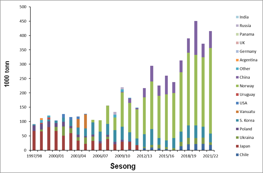
The Antarctic krill (Euphausia superba) fishery started in the early 1970s and peaked in the late 1980s with catches up to 500,000 tons per year, by USSR and Japanese vessels operating in several areas of the Southern Ocean. The fishing for Antarctic krill is currently concentrated within the Southwest Atlantic sector of the Southern Ocean (Commission on the Conservation of Antarctic Marine Living Resources (CCAMLR) subareas 48.1, 48.2, 48.3 and 48.4. A fixed precautionary annual catch limit for this sector was set to 620,000 tons (termed the ‘trigger level’) by CCAMLR in 1991 (CCAMLR Conservation Measure 51–01). The total krill catch for the 2021/22 season was 415 510 tons (35% taken in 48.1, 46% in 48.2, 19% in 48.3 and 0 in 48.4). The overall catch proportion taken by the Norwegian krill industry represented 72%, the Chinese vessels caught 14%, South Korea 7%, Chile 5%, and Ukraine 2% (Figure 1).
Figure 1. Annual total catch per flag state in the CCAMLR subareas 48.1, 48.2, 48.3 and 48.4, since 1997/98 to 2021/22 (data source: CCAMLR.org).
Two large-scaled acoustic trawl surveys have been executed in the Southwest Atlantic sector of the Southern Ocean (subarea 48.1-48.4), calculating a total biomass of krill in these fishing areas to be 62.6 Mt in 2019 (Krafft et al., 2021), which was similar to the synoptic survey in 2000 (60.3 Mt; CCAMLR, 2010). Regular monitoring on meso-scale of krill distribution and demographic composition in these fishing areas, have been carried out by the US Antarctic Marine Living Resources program (AMLR) since 1996 (Reiss et al., 2008), in the Bransfield Strait and Elephant Island area (subarea 48.1). During recent years also Chinese and Korean vessels survey these same AMLR transects. Previously these surveys were made during the austral summertime but presently also during the austral winter. The British Antarctic Survey run an annual acoustic survey off the South Georgia Islands (“Western core-box” subarea 48.3, since 1997 (Fielding et al., 2014) during the summer season.
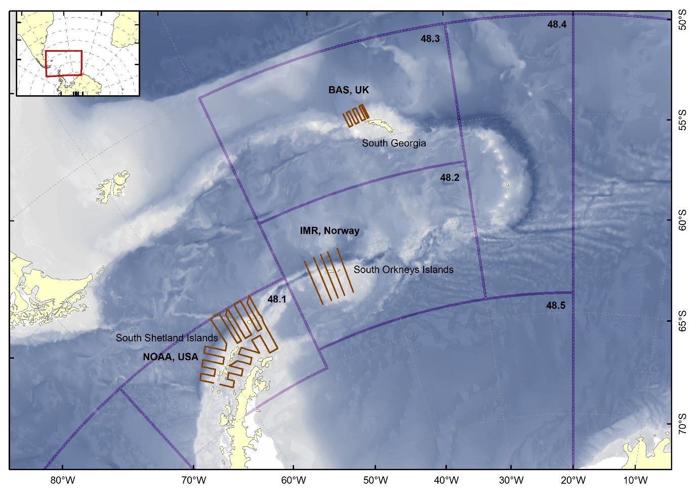
A Norwegian fishing company offered to carry out an annual krill monitoring survey commencing in 2011, for as long as they have commercial activity in the Southern Ocean (Jensen et al. 2010). Through discussions in CCAMLR WG-EMM (Working Group on Ecosystem Monitoring and Management) in 2010, it was agreed that the survey could be carried out in the CCAMLR statistical Subarea 48.2 according to similar standards as the annual scientific surveys undertaken in 48.1 and 48.3 and that the surveys should be executed with scientists from the Institute of Marine Research, Norway. The three surveys could form an integrated monitoring effort extending across the Scotia Sea (Figure 2), linking three of the areas with highest concentrations of krill and highest fishing activity. The results will help evaluate and develop the management of the krill fishery (Hill et al., 2016).
The first annual survey was carried out in January/February 2011 using the FV ’Saga Sea’ (Aker Biomarine ASA). The results and study design from this survey was presented at the CCAMLR WG-EMM in 2011. The original survey design (suggested during WG-EMM 2010) consisted of six parallel north-south bound transects extending 100 nmi. During this first survey season it was recognized a need to extend the monitoring effort covering the waters over the shelf edge, north of the South Orkney archipelago, where most krill in this region traditionally aggregate. During the WG-EMM meeting in 2011 it was agreed to extend the survey transects 20 nmi northwards and to omit the westernmost transect line from the 2011 survey. Before the survey in 2014, it was also agreed to extend the transect lines further to the south to cover the northern part of the Marine Protected Area south of the South Orkney Islands, and the design has since remained unchanged (Figure 2).
Figure 2. CCAMLR Statistical Reporting Areas 48.1–48.3 with transect lines regularly surveyed for Antarctic krill abundance and demography.
Results and activities from these annual South Orkney surveys are regularly reported to WG EMM (e.g. Krafft et al., 2018, Skaret et al., 2019) and are published in the primary literature (e.g. Krafft et al 2018, 2019, Skaret et al. 2023). This report presents the survey activities from the 2023 season off the South Orkney Islands including results from acoustic recordings, taxonomic sorting of trawl catches and krill predator sighting data collected during daylight hours along the transects. A pilot study using flying drones were also made to explore the potential for providing information on the distribution of whale groups over a wider area. Also, a land-party was deployed on Powell Island to tag penguins for satellite tracking of foraging movements and to study potential overlap with fishing activities.
Material and Methods
Survey design, area, and vessel
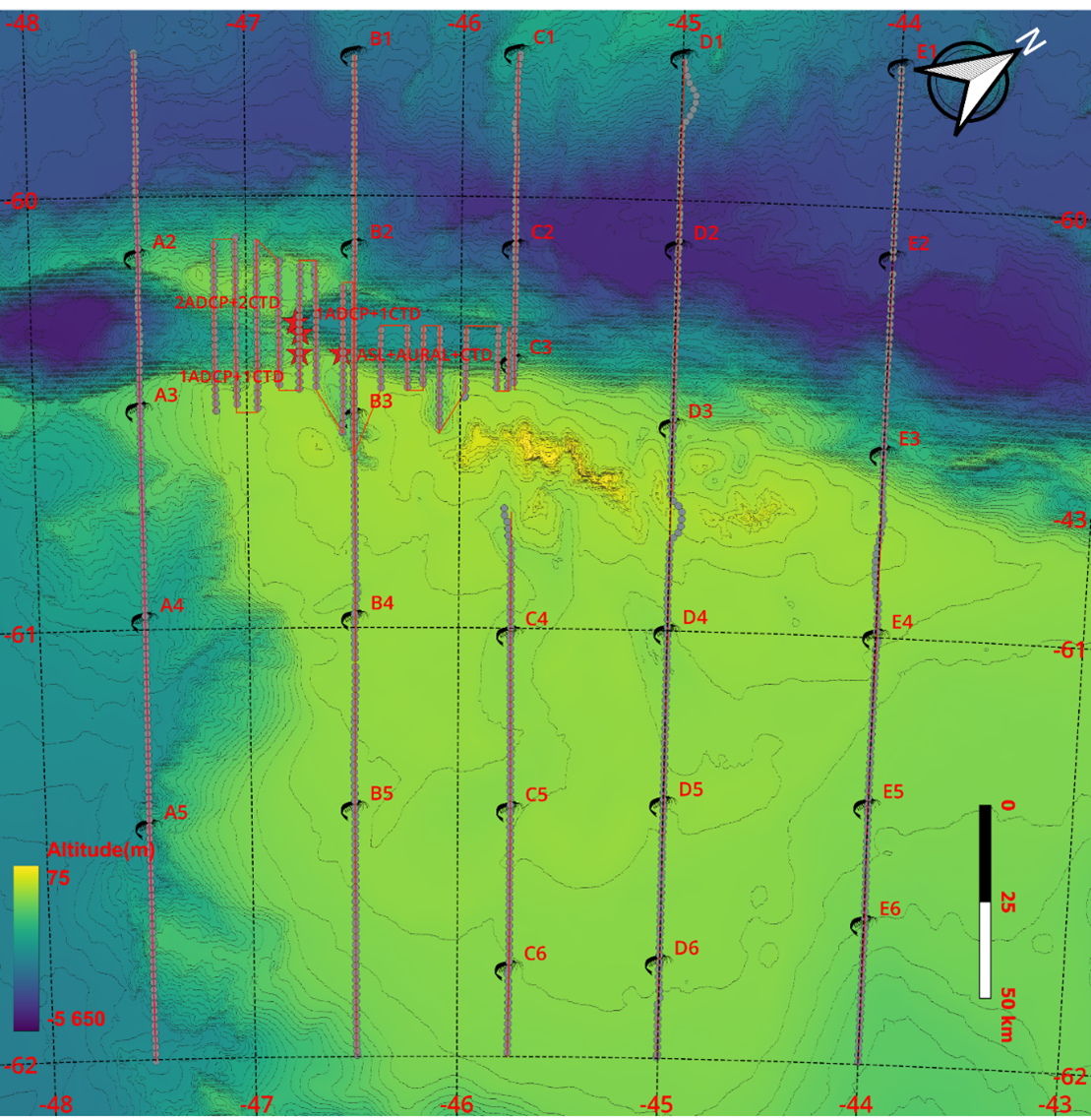
The Cargo vessel “Antarctic Provider” (Aker Biomarine AS) departed Puerto Williams, Chile, on the 23. January. On the 24. February the survey ended by reaching port in Montevideo. The survey design covers 60 360 km2 of the waters around the South Orkney Islands and includes five parallel transects extending from the northernmost waypoints at 59.67°S and southernmost waypoint at 62.00°S. Longitudes for transects 1 through 5 are at 44°W, 45°W, 45.75°W, 46.5°W and 47.5° W, respectively.
In addition, a small Shelf edge stratum at 2368 km2 was covered with a denser transect grid. The Shelf edge stratum covers the locations with the highest historical krill catches. The acoustic sampling effort is higher than in the main strata, but otherwise, the design is the same (Figure 3).
Figure 3. Summary of the 2023 krill monitoring survey lines covered with the 27 trawl stations (A2 to E6) carried out. Four moorings were deployed as denoted by the red stars.
Acoustic data collection
Vessel mounted echosounders
During the survey ‘Antarctic Provider’ was equipped with Simrad EK80, 18 kHz and EK60 echo sounders operating at 38, 70, 120 and 200 kHz.
The echosounders were calibrated while at anchor off Signy Island using the standard sphere calibration method (Foote et al., 1987). The echo sounder was operating with a ping interval at or close to 1 per second. Nominal vessel speed during surveying is 10 knots and could be kept during most of the survey. Acoustic data were collected down to 600 m on all five frequencies. Other transceiver settings are specified in Table 1.
Table 1. Specification of transceiver settings on ‘Antarctic Provider’ applied during the 2023 survey.
Transducer type
ES18
ES38-7
ES70-7C
ES120-7C
ES200-7C
Transmitted power (W)
1600
2000
750
250
2000
Pulse duration (ms)
1.024
1.024
1.024
1.024
1.024
Absorption coefficient (dB km-1)
3.48
10.21
17.89
25.83
39.85
Sound speed (ms-1)
1452
1452
1452
1452
1452
Sample distance (m)
0.186
0.0348
0.186
0.186
0.186
Two-way beam angle (dB)
-17
-20.7
-20.7
-20.7
-20.7
SV transducer gain (dB)
21.07
26.99
26.62
26.56
25.97
SA-correction
-0.47
-0.12
-0.33
-0.36
-0.33
Acoustic moorings
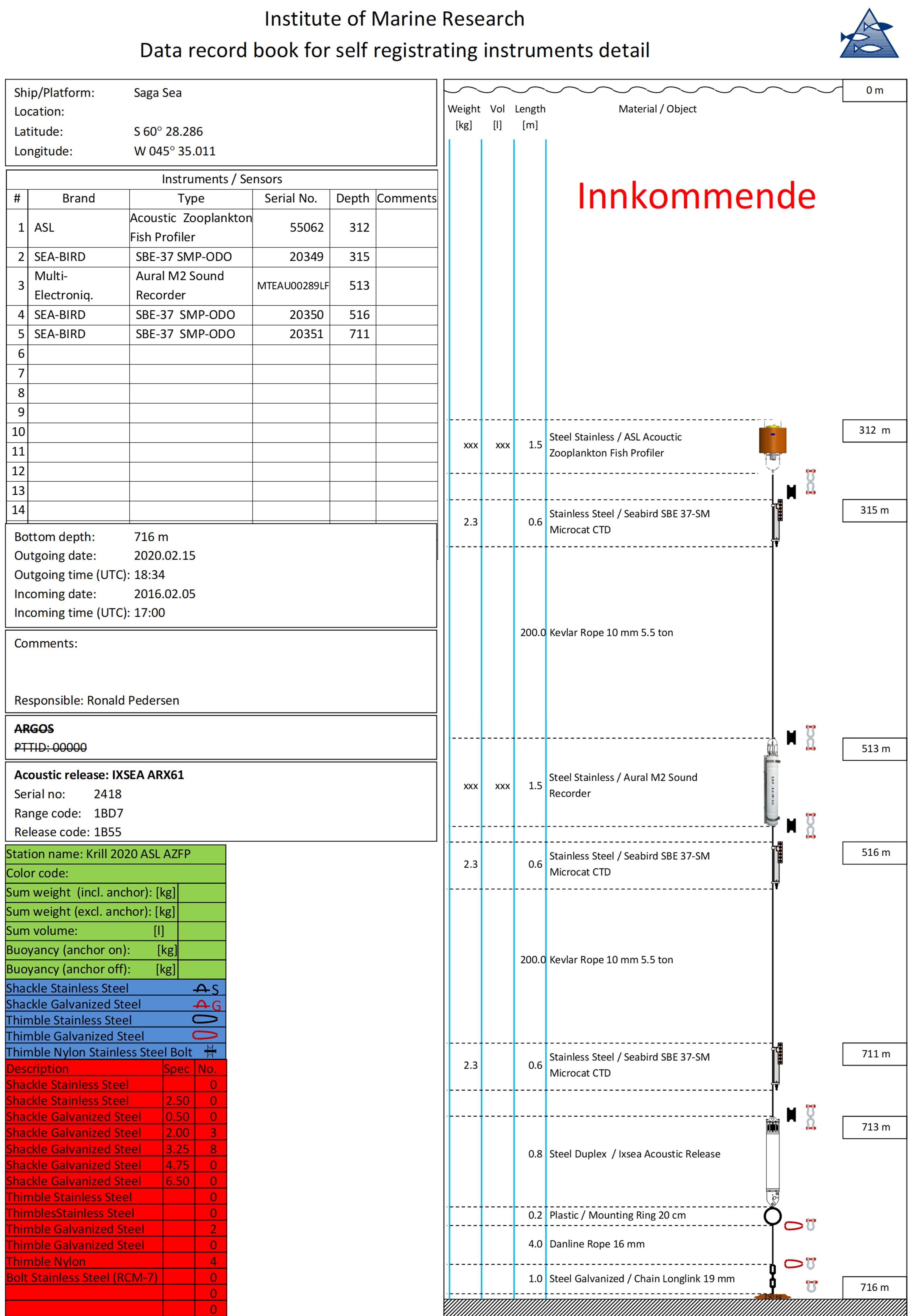
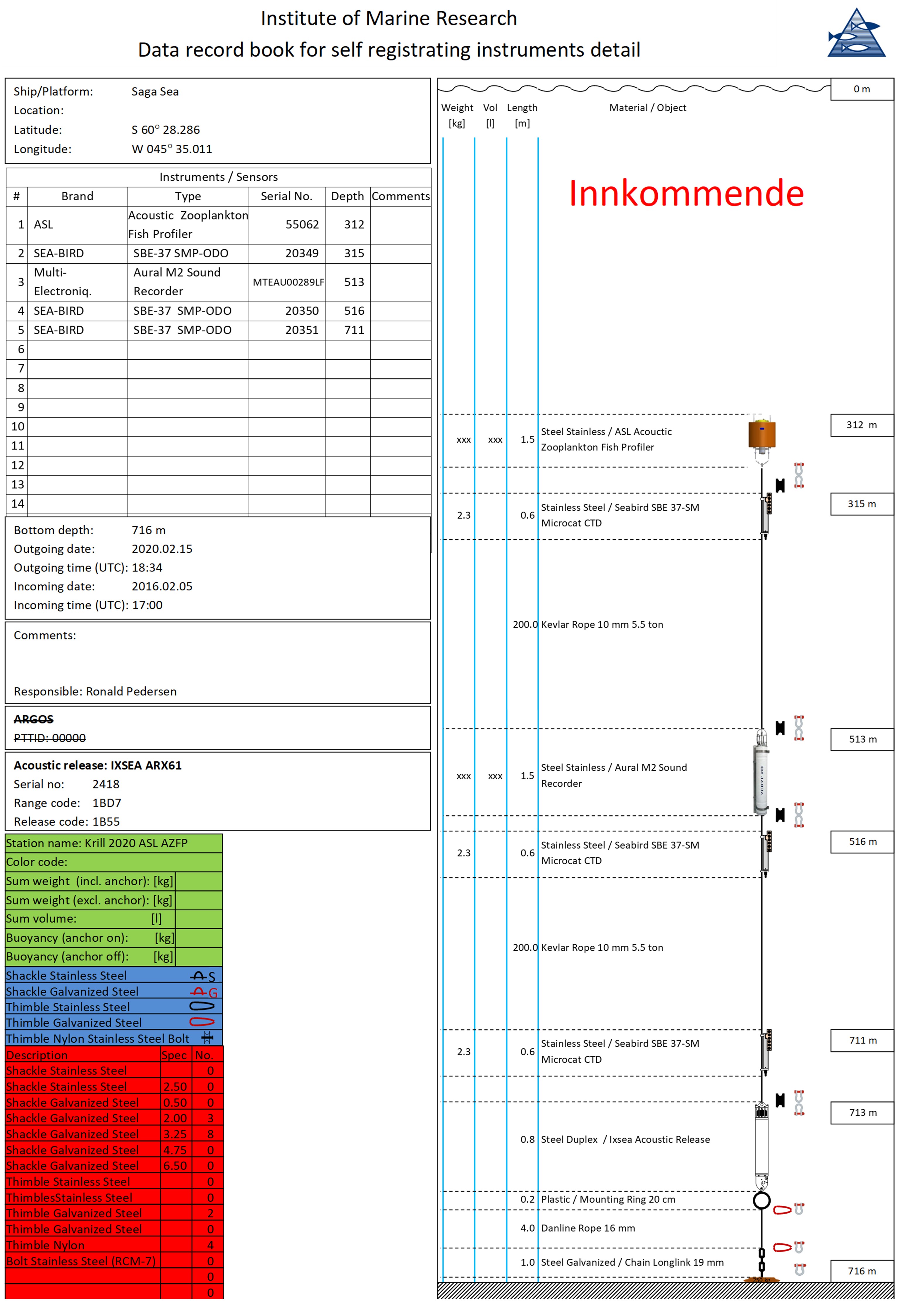
An Aural hydrophone was deployed in 2020 for passive recording of marine mammal vocalization in parallel with an ASL echosounder and a Seabird CTD, that were successfully retrieved at position S 60° 24.28.286 and W 045° 35.011 (Appendix 1).
After downloading data, batteries were changed, the unit was reprogrammed and refurbished. The Aural hydrophone was redeployed together with the ASL and CTD at S 60°21.917 and W 046° 33.365 (Appendix 2)
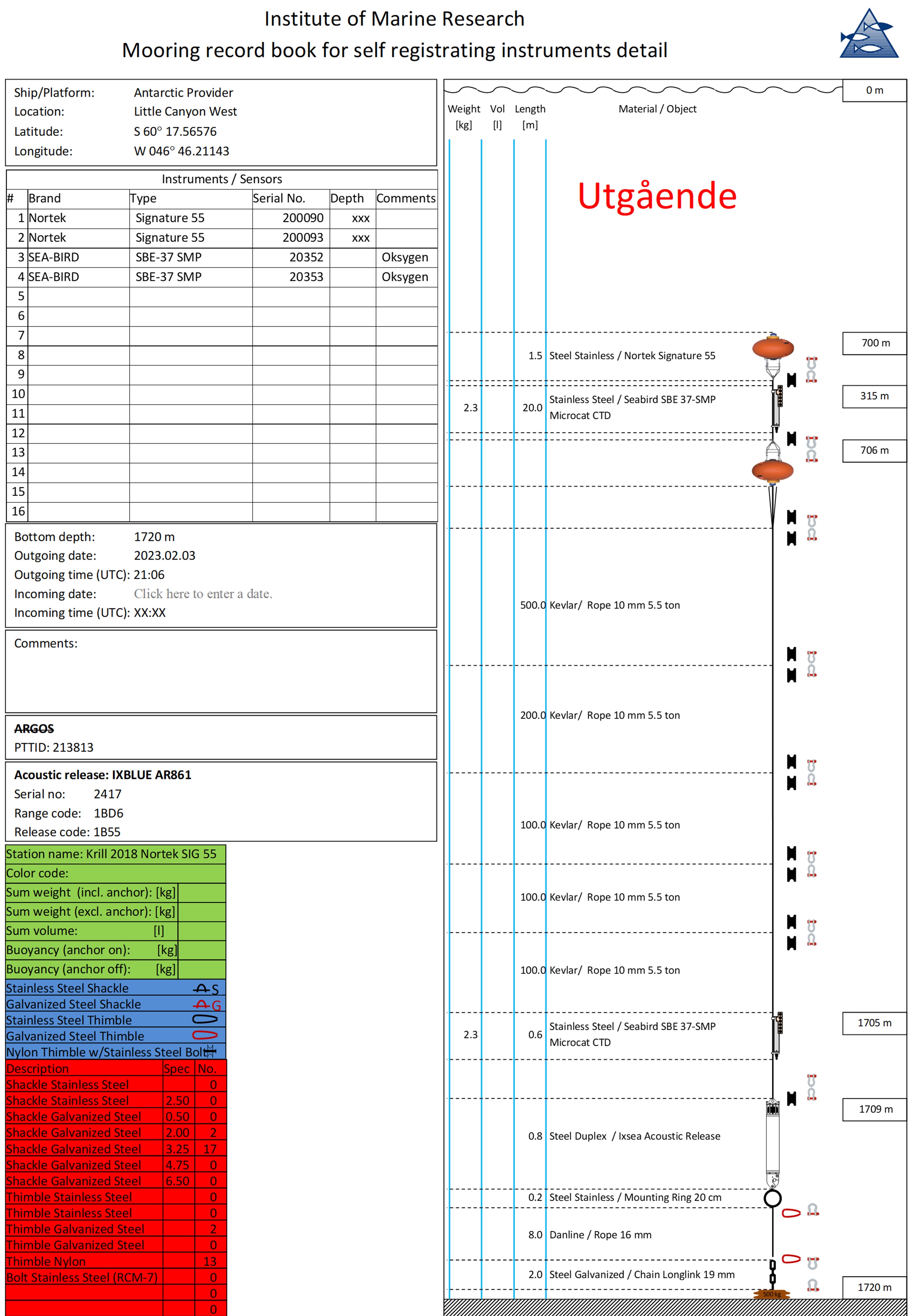
A mooring containing two NorTek Signature 55 combined echo sounder and Acoustic Doppler Current Profiler (ADCP), with one pointing upwards and the other downwards, and two CTDs were deployed at S 60° 17.56576 and W 045° 46.21143 (Appendix 3).
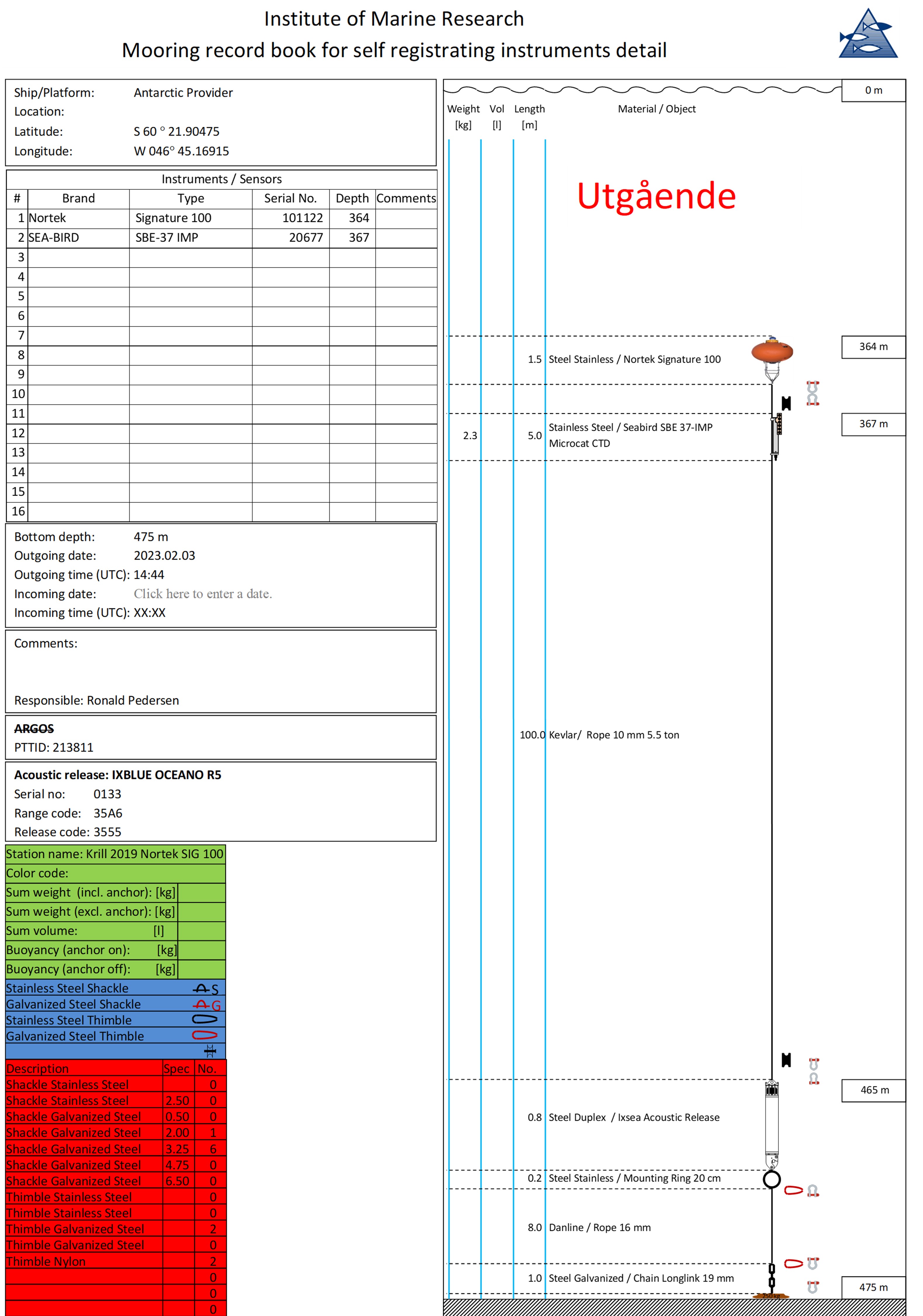
A second mooring containing a Nortec Signature 100 and a CTD was deployed at S 60° 21.90475 and W 046° 45.16915 (Appendix 4).
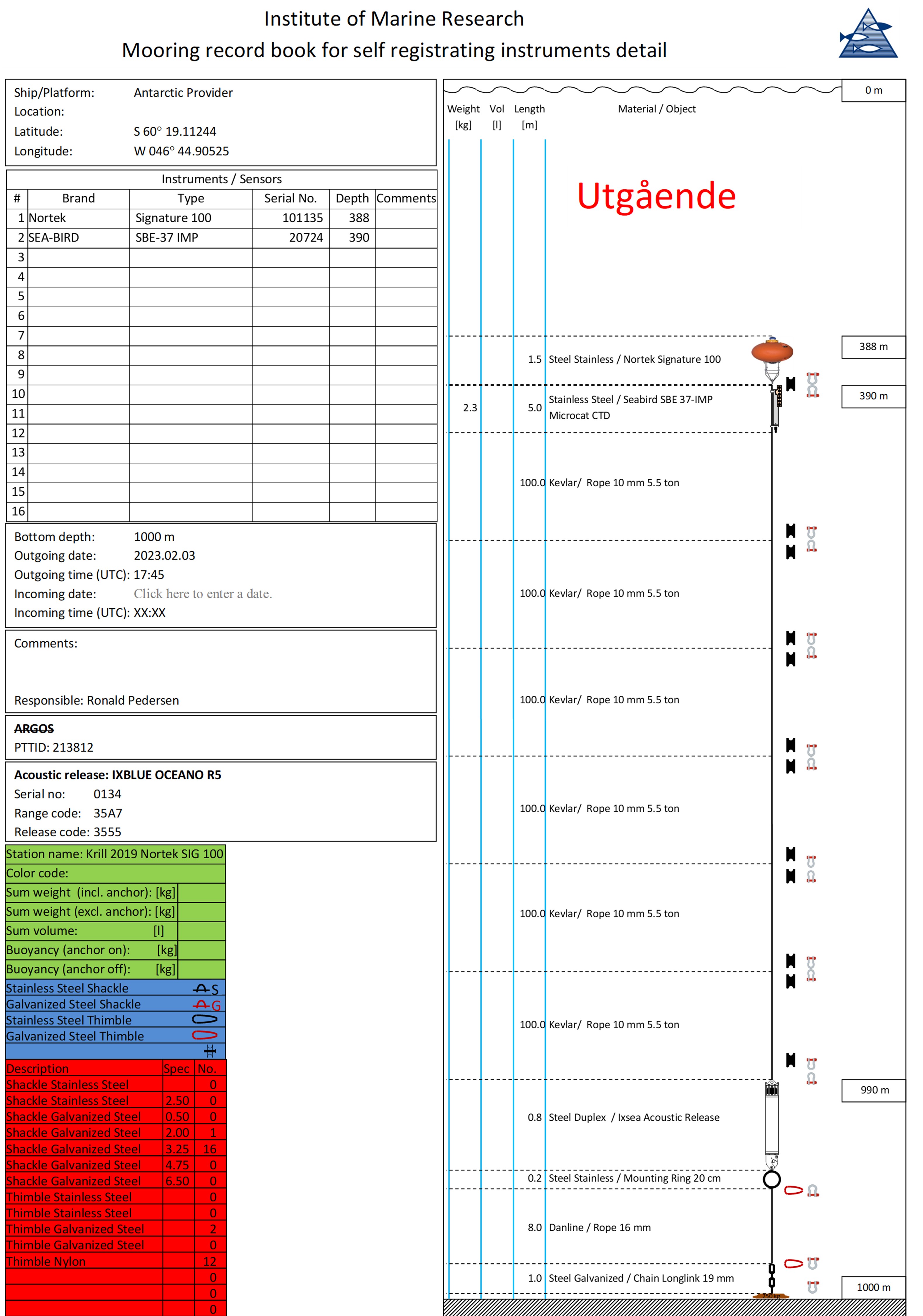
The third mooring contained a Signature 100 and a CTD deployed at S 60° 19.11244 and W 046° 44.90525 (Appendix 5).
Acoustic data analyses
Discrimination of targets
In this work, we applied the standard swarm-based technique for krill discrimination on 120 kHz data using an Echoview work template, which includes noise removal filters, a swarm detection filter and an integration module (CCAMLR, 2017). Swarm detection was implemented using the Large Scale Survey System (LSSS) computer program (Korneliussen et al., 2016).
Target strength prediction
The NASC were converted to biomass density (gm-2) using the SDWBApackage2010 (Conti and Demer, 2006; SG-ASAM 2010; Calise and Skaret, 2011) according to the CCAMLR protocol. The model was parameterized according to Table 1, or if nothing else specified according to Calise and Skaret (2011).
The predicted target strengths were used to calculate weighted conversion factors (CF) from NASC-values to biomass density
where f is the frequency of a specific length group (i) and W(TL) is weight at total length, which was calculated following Hewitt et al. (2004):
σ(TL) is the backscattering cross-section at a specific total length and was calculated using the full SDWBA model.
Estimation of biomass
Based on the average biomass density for each nautical mile, a weighted biomass density for each transect line could be calculated and the sampling variance from the averages of each transect line according to Jolly and Hampton (1990).
Biological sampling
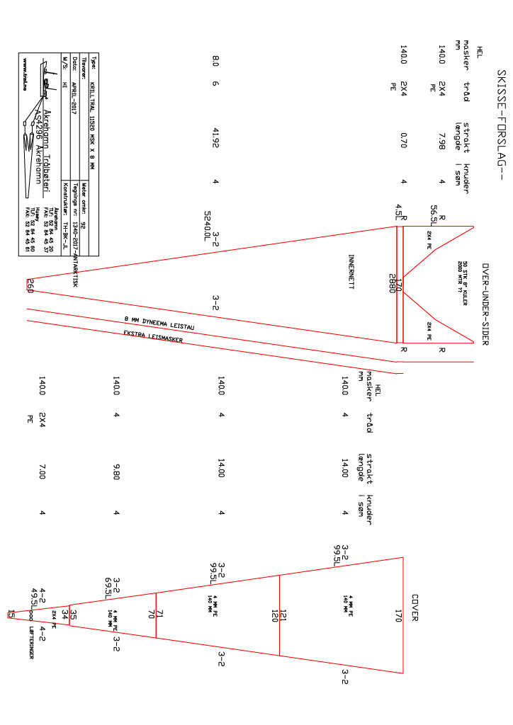
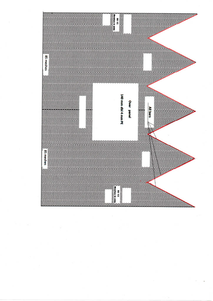
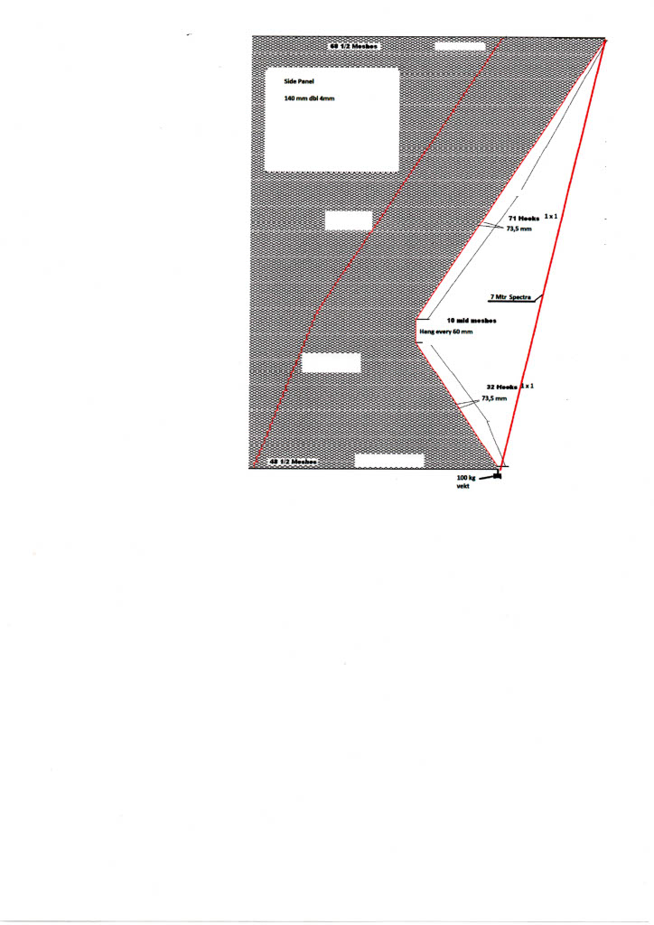
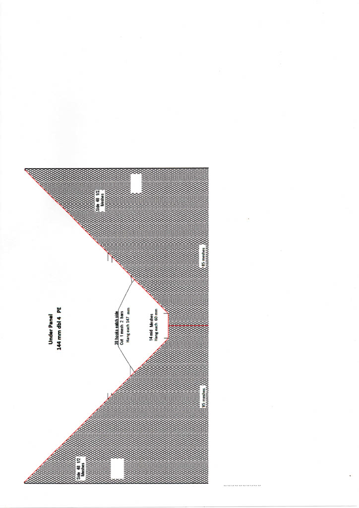
The survey design included trawl stations spaced ~20–25 nautical miles apart along the set parallel north-south oriented transect lines (Figure 1). The standard survey trawl used was 42 m long, with a 36 m2 mouth opening, constructed of 7 mm (stretched) diamond shaped meshes from mouth to rear, or a 3 mm light opening. The trawl was towed using a 6 m wide steel beam with 200 kg weights at each lower wing tip to ensure fast deployment to depth and the best possible geometric stability of the trawl during sampling (see Appendix 6, 7, 8 and 9 for trawl and front part design).
At each station the trawl was lowered vertically from surface to ~200 m depth (or ~20 m above bottom if the water was < 200 m) and then hauled in at ~1.5 knots (includes both vessel and wire speed). When landed on the trawl deck, the cod end was opened, and catch was removed. Thereby the towing rig was hung from a crane and flushed on deck to wash out biological remains stuck in the net. The macro zooplankton and micronekton were sorted, identified to species or to the nearest possible taxonomic group, and weighed. For E. superba, the length of individual krill was measured (± 1 mm) from the anterior margin of the eye to the tip of telson excluding the setae, according to the “Discovery method” used in Marr (1962). Sex and maturity stages of E. superba were determined on fresh material using the classification methods outlined by Makorov and Denys (1981). In brief, juveniles are classified due to their lack of visible sexual characteristics. Males were divided into three sub adult stages: MIIA1, MIIA2 and MIIA3 and two adult stages: MIIIA and MIIIB, females were divided into one sub adult stage: FIIA and five adult stages: FIIIA, FIIIB, FIIIC, FIIID and FIIIE (see Krafft et al.2015 for further details).
Hydrographical sampling
A Seabird CTD sensor was mounted in an open metal frame for protection and welded on the trawl beam to obtain profiles of temperature and salinity during the trawl hauls.
Marine predator observations
Marine mammal observations were carried out by dedicated observers during daylight hours. The observer was located on the bridge and continuously scanned the starboard forward quarter visually (0 – 90°), binoculars were used for species identification. Angle were estimated using a drawn angle board. Distance estimation was aided by using the reticles in the binoculars that marked one milliradian per line. Together with the platform and observer height (20.3+1.7m), each reticles line from the horizon marked a known distance.
Observations were only recorded on straight sections of the vessel track with a nominal vessel speed of 10 knots. The vessel GPS track and logged effort were recorded with custom software on a touchscreen computer. For each observation the species, time, location, distance, angle, visibility and number of individuals were noted.
Pilot study using flying drones for estimating whale size structure
Size structure of individual whales was assessed using drones (Unmanned Aerial Systems (UAS)) providing overhead photogrammetry of whales. Data collection was carried out between January 28th and February 10, from the Aker Biomarine A/S F/V Antarctic Endurance during normal fishing operations off the South Orkney Islands.
The drone operations were carried out using a Freefly Alta 6 equipped with a gimbal-stabilized camera system containing:
1. Sony A6000 24 MP camera, equipped with a 35mm lens, used in particular for photogrammetry of body size/condition
2. Runcam Hybrid 2 dual FPV and HD video camera, used for locating animals and to provide video-based general contextual data
3. Lightware SF 11-C laser altimeter, to provide accurate altitude information for body photogrammetry analyses
4. GoPro Fusion 360-degree video camera for wide-field contextual and spatial distribution information
Additional material was collected using a DJI Mavic 2 Enterprise Dual.
Operations were carried out from the open deck area below and in front of the vessel bridge. The Freefly Alta 6 was operated by two persons: one drone pilot and one gimbal/camera operator, while the Mavic 2 Enterprise Dual was operated by one person controlling both the aircraft and the camera.
Still images collected from directly overhead individual whales were used to estimate body morphometrics using the custom-written Python package morphometrix (Torres & Bierlich, 2020; https://github.com/wingtorres/morphometrix.git). Briefly, morphometrix is an interactive system that allows the user to: 1. Fit a bezier curve (or a set of straight line segments) between the snout and tail notch in order to estimate body length, 2. Input a desired number of equally spaced sections along the length at which body width estimates can be obtained, 3. optionally, the area of user-defined objects (e.g. appendages, skin coloration patches etc.) can be calculated. All measurements are automatically converted from pixel coordinate values to real-world measurements by inputting the camera lens specifications and the altitude recorded by the laser altimeter.
Penguin foraging
The two-person field-teams initial plan was to deploy in early December 2022 to Monroe Island on the northwest corner of Coronation Island in order to replicate the data collected during the first SUFIANT field season; specifically, to collect acoustic data on krill density and distribution across the areas that krill-dependent chinstrap penguins (Pygoscelus antarcticus) forage. These data, supplemented by animal-borne High Definition video data of at-sea feeding, are currently being used to build a near-real-time monitoring system whereby the feeding success of individual penguins can be quantified relative to the abundance of prey in their foraging area.
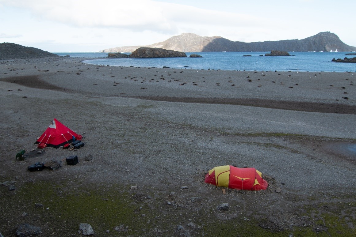
Figure 4. Remote field camp operated by the research team on Powell Island. As well as hosting a large number of chinstrap penguin breeding colonies, many hundreds of adult male Antarctic fur seals arrive on the island throughout January, travelling from South Georgia at the completion of the summer breeding season.
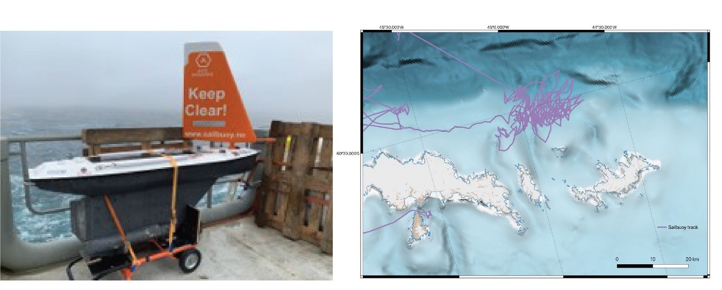
A combination of ship delay and bad weather necessitated a change in this plan, deploying to Powell Island on 6th January 2023 in a field camp on the southern end of the island (Figure 4). Given that the research team had worked on Powell Island previously, prior knowledge of the at-sea behaviour of chinstrap penguins allowed the team to deploy a surface ROV (Sailbuoy) in the general vicinity of where the penguins were known to feed (Figure 5) which remained in place collecting acoustic data on krill density and distribution for the 21days the field team were in place.
Figure 5. Surface autonomous ROV (“Sailbuoy”) deployed in the area where chinstrap penguins were known to forage at Powell Island in January 2023. The vehicle remained in place collecting acoustic data on krill density and distributions for approximately 3 weeks despite severe weather.
Results
Acoustics
Acoustic survey estimates of krill distribution and biomass
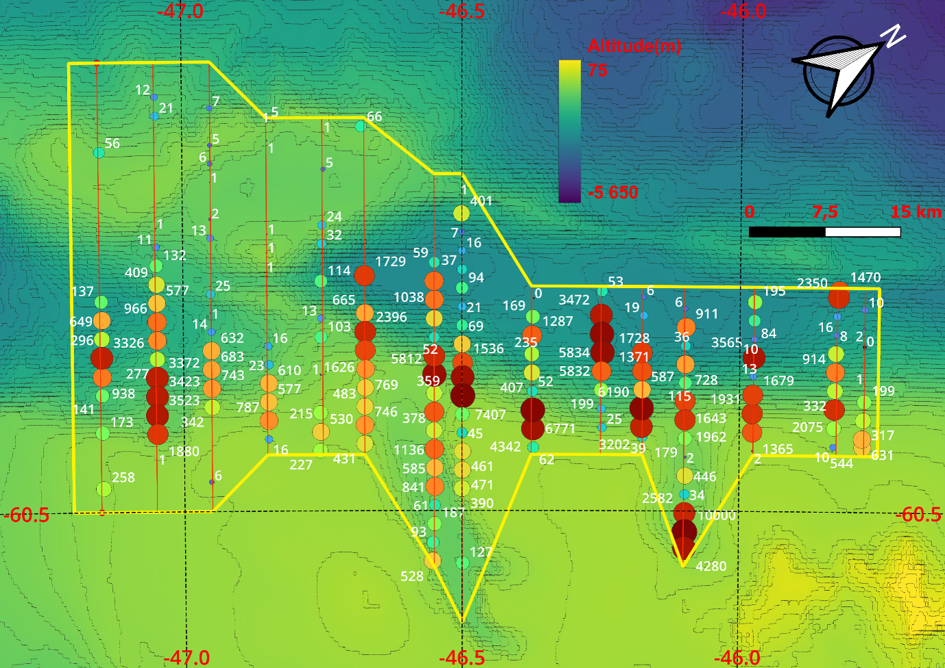
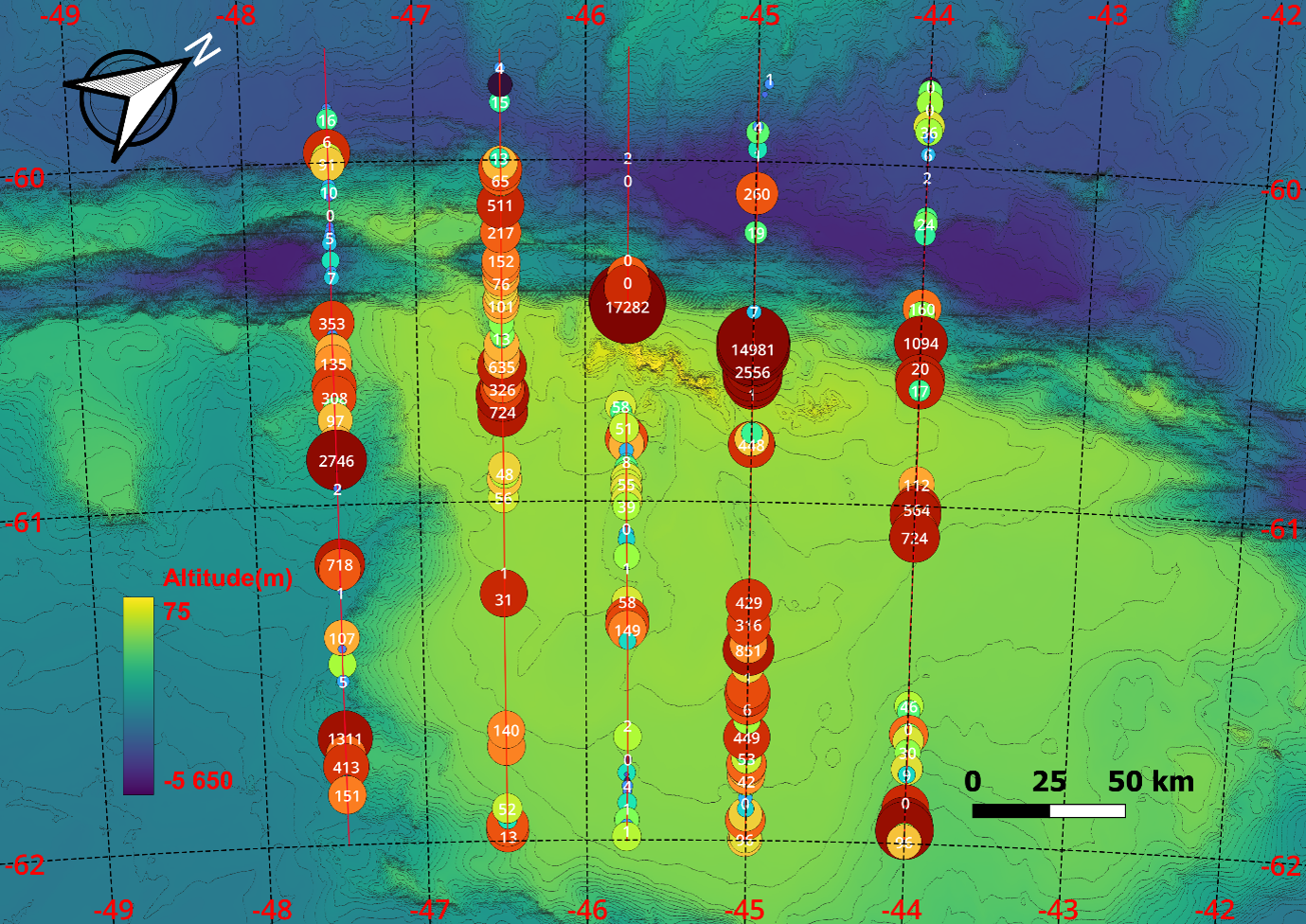
The distribution of acoustic backscatter allocated to krill is shown Figure 6. The highest NASC-values allocated to krill were observed around the shelf edge and canyons. There were lower values in the northern part of the covered area than previously observed. The krill length distributions are obtained by trawl samples (Figure 8). The biomass estimates are shown in Table 2.
(a)
(b)
Figure 6. Distribution of Nautical Area Scattering Coefficients (NASC; m2/nmi2) allocated to E.
superba (red) and other targets (grey) from the 120 kHz recordings. Log distance is 1 nautical mile. The symbols are not linearly scaled due to space. (a) the Shelf edge stratum, (b) the overall stratum.
Table 2. Summary tables of krill biomass estimation using the swarms method from all surveys (Skaret et al., 2023: 2011-2020 and this survey 2023 2023. 2a summarize results from the Shelf edge stratum, 2b summarize data from the overall stratum.
2a
Year
Freq
Density (g/m2)
BM (mill tonn)
CV
2011
2012
2013
2014
2015
38
31.6
0.07
0.24
2016
2017
2018
2019
120
217.6
0.52
0.19
2020
38
62.0
0.15
0.27
2023
120
202.9
0.48
0,23
2b
Year
Freq
Density (g/m2)
BM (mill tonn)
CV
2011
120
62.6
3.78
0.36
2012
120
128.8
7.77
0.35
2013
38
76.5
4.62
0.30
2014
38
28.5
1.72
0.19
2015
38
49.3
2.98
0.49
2016
120
23.2
1.40
0.29
2017
120
69.4
4.19
0.25
2018
120
27.2
1.64
0.29
2019
120
38.8
2.34
0.14
2020
38
62.6
3.78
0.36
2023
120
36.7
2.21
0.51
Biological sampling
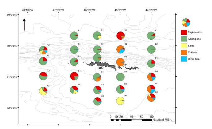
A total of 27 trawl stations was successfully completed during the survey (Figure 7), of which one (Station E2) was only sampled from 90m depth due to bad weather conditions. The total catch was dominated by euphausiids (40,0%), amphipods (28,3%) and salpa (25,6%). Four species of euphausiids were identified: E. superba, Thysanoessa macrura, E. frigida and E. tricantha. E. superba was present at 24 of the stations, however most of its catch was concentrated at station B2, which accounted for 96,7% of total sampled E. superba. The amphipod T. gaudichaudi was present at 26 stations and was the most frequent taxa occurring in the trawl samples. The rest of the biomass consisted of Cnidaria (3,9%), Teleostei (1,3%), Calanoids (0,2%), and other taxa (0,8%), where the most occurring species and taxa were Diphyes sp. Chaetognatha, Polychaeta, Mysidae, and Chionodraco spp.
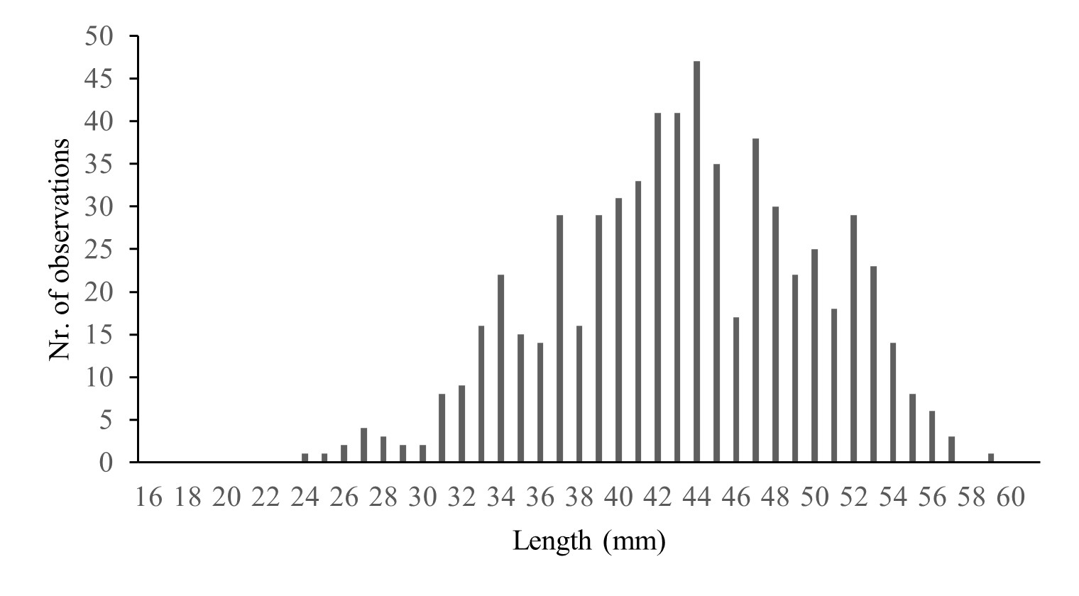
The average body length of E. superba was 45.79 ± 5.4 (SD) mm, and the range was 24-59 mm (Figure 8). The demographic composition of E. superba caught in the trawl was dominated by younger specimens, with the highest proportion of measured E. superba centered around the juvenile stage (14,8%), subadult females (FIIB: 23,2%, FIIIA:11,5%), and subadult males (MIIA2:13,7%). There was also a considerable proportion of adult males in the samples (MIIIB: 13,9%) (Table 3), these were mainly caught at stations in the north-western part of the transect (stations A1, B1, B2, B3), while gravid females (FIIIC: 5,8%, FIIID: 4,6%) were found mainly in the north-western and south-eastern stations (stations A2,B1,B2,B3 and D5,D6,E4,E6).
Figure 7: The most common taxonomic groups (Euphausiids, Amphipods, Salpa, Cnidaria, and other taxa) in terms of proportional catch weight.
Figure 8: Length distribution of E. superba caught during the survey.
Table 3: Sexual maturation stages, number of observations, proportion (%), and mean length of E. superba.
Stage
N
Proportion
Mean ± SD
Juvenile
94
14.8
34.6 ± 4.8
FIIB
147
23.2
40.3 ± 3.2
FIIIA
73
11.5
46.4 ± 3.0
FIIIB
8
1.3
46.4 ± 3.9
FIIIC
37
5.8
49.5 ± 3.4
FIIID
29
4.6
51.0 ± 3.3
FIIIE
14
2.2
50.6 ± 3.9
MIIA1
39
6.2
37.8 ± 3.5
MIIA2
87
13.7
42.5 ± 2.9
M!!A3
14
2.2
47.5 ± 3.6
MIIIA
4
0.6
52.0 ± 1.6
MIIIB
88
13.9
50.8 ± 2.9
Total
634
Hydrography
The hydrographical profiles from the survey area based on the trawl mounted CTD are shown in figure 9. A thermocline was observed around 50-60 m in most of the trawl stations, it increased to 100 m at the stations A4 and A5, there was no obvious thermocline at B1, B3, D3 and D4, and the halocline depth was observed similar with the thermocline.
Figure 9. Hydrographical profiles from the ctd-casts with temperature in black and salinity in blue.
Marine predator observations
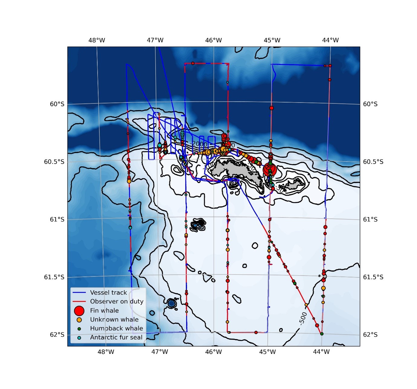
The conditions for predator observing were average during most of the survey. There was swell and/or wind and also quite frequent periods of fog which limited the visual range. A total of 570 Fin whales (Balaenoptera physalus), 46 Antarctic fur seals (Arctocephalus gazella), 30 Humpback whales (Megaptera novaeangliae) and 177 unknown whale species were sighted (Figure 10).
Figure 10. Vessel track, observations efforts and marine mammal sightings.
Drone observations
A total of 1314 images were deemed sufficient for morphometrics measurements as well as individual identification. In total, we identified 43 individual whales, of which 12 were humpback whales and 31 were fin whales. While comprehensive morphometric analyses have not yet been carried out, preliminary analyses revealed a widespread in body sizes for both species, and we also encountered several mother/calf pairs for both humpback and fin whales.
Despite the prevalence of relatively poor weather conditions and the operational constraints imposed by normal fishing operations restricting the work to some degree, we were able to collect useful data on a total of 12 days out of the 19 days onboard FV Endurance. Comprehensive analyses of these data, in combination with data on krill biomass from the onboard echosounders will allow to examine variations in whale presence and relative abundance in relation to variations in krill biomass. This will also form the basis for the development of functional response estimates of krill consumption by whales. By combining this with body size estimates from the drone-based morphometrics, as well as abundance estimates from line transect distance sampling carried out during the simultaneous wider-area krill survey, we will provide estimates of krill consumption by the key cetacean krill consumers in the area; fin and humpback whales.
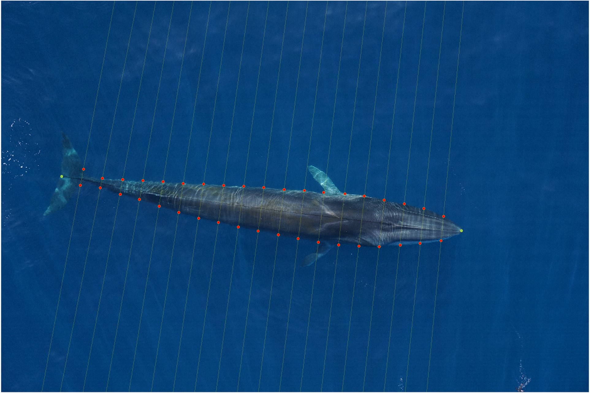
Figure 11. Example of morphometrics measurements of a fin whale obtained using the morphometrix package. Note also the coloration patterns above the right eye, and the distinct chevron pattern on the back the pectoral fins. These were used to identify individuals and thus determine the identity of the measured animals. This particular image, taken from an altitude of 46.7 meters, gave an estimated total body length of 21.6 meters, greatest width of 2.7 meters, and a volume of 64.6 cubic meters. Assuming a body density similar to that of freshwater, this yields an estimated body weight of about 64 tons.
Acknowledgements
This work is financed by the project KRILL , pno. 14246 (IMR, Ministry of Trade, Industry and Fisheries), SUFIANT (Research Council of Norway and Aker Biomarine ASA), Antarctic Wildlife Research fund and the Ministry of Foreign Affairs. We extend our gratitude to the Aker Biomarine AS for providing ‘Antarctic Provider’ and its crew to disposal for this research survey free of charge. We are most grateful to the captain, officers, and crew on board for all the help provided during the survey.
References
Calise, L. and Skaret, G. 2011. Sensitivity investigation of the SDWBA Antarctic krill target strength model to fatness, material contrasts and orientation. CCAMLR Science, Vol. 18 (2011): 97–122
CCAMLR (Convention on the Conservation of Antarctic Marine Living Resources). (2010) Report of the 29th meeting of the scientific committee, Hobart, TAS, Australia, 25-29th October, 2010. SC-CAMLR- XXIX. CCAMLR, Hobart, TAS, Australia.
Conti, S.G. and D.A. Demer. 2006. Improved parameterization of the SDWBA for estimating krill target strength. ICES Journal of Marine Science, 63 (5): 928-935.
Fielding, S., Watkins, J.L., Trathan, P.N., Enderlein, P., Waluda, C.M., Stowasser, G., Tarling, G.A. & Murphy, E.J. 2014. Interannual variability in Antarctic krill (Euphausia superba) density at South Georgia, Southern Ocean: 1997–2013. ICES Journal of Marine Science, 71: 2578–2588.
Foote, K.G., H.P. Vestnes, D.N. MacLennan and E.J. Simmonds. 1987. Calibration of acoustic instruments for fish density estimation: a practical guide. ICES Cooperative Research Report, 144, 69 pp.
Hewitt, R. P., Watkins, J., Naganobu, M., Sushin, V., Brierley, A. S., Demer, D., Kasatkina, S., Takao, Y., Goss, C., Malyshko, A., Brandon, M., Kawaguchi, S., Siegel, V., Trathan, P., Emery, J., Everson, I., and Miller, D. 2004. Biomass of Antarctic krill in the Scotia Sea in January/February 2000 and its use in revising an estimate of precautionary yield. Deep-Sea Research Part II-Topical Studies in Oceanography, 51: 1215-1236.
Hill SL, Atkinson A, Darby C, Fielding S, Krafft BA, Godø OR, Skaret G, Trathan P, Watkins J. 2016. Is current management of the Antarctic krill fishery in the Atlantic sector of the Southern Ocean precautionary? CCAMLR Science 23:31-51
Jensen N, Nicoll R, Iversen SA (2010) The importance of obtaining annual biomass information in CCAMLR Sub-area 48.2 to inform management of the krill fishery. WG-EMM-10/9, 5 pp
Jolly GM, Hampton I (1990) A stratified, random-transect design for acoustic surveys of fish stocks. Canadian Journal of Fisheries and Aquatic Sciences 47: 1282–1291.
Krafft BA, Krag LA, Knutsen T, Skaret G, Jensen KHM, Krakstad JO, Larsen SH, Melle W, Iversen SA, Godø OR. Summer distribution and demography of Antarctic krill (Euphausia superba) (Dana, 1852) (Euphausiacea) at South Orkney Islands, 2011–2015. Journal of Crustacean Biology, submitted 2018.
Krafft BA, Macaulay GJ, Skaret G, Knutsen T, Bergstad OA, Lowther A, Huse G, Fielding S, Trathan P, Murphy E, Choi S-G, Chung S, Han I, Lee K, Zhao X, Wang X, Ying Y, Yu X, Demianenko K, Podhornyi V, Vishnyakova K, Pshenichnov L, Chuklin A, Shyshman H, Cox MJ, Reid K, Watters GM, Reiss CS, Hinke JT, Arata J, Godø OR, Hoem N. 2021. Standing stock of Antarctic krill (Euphausia superba Dana 1850 (Euphausiacea)) in the Southwest Atlantic sector of the Southern Ocean, 2019. 2021. Journal of Crustacean Biology. 41:1-17. https://doi.org/10.1093/jcbiol/ruab046
Krafft BA, Krag LA, Knutsen T, Skaret G, Jensen KHM, Krakstad JO, Larsen SH, Melle W, Iversen SA, Godø OR. 2018. Summer distribution and demography of Antarctic krill (Euphausia superba) (Dana, 1852) (Euphausiacea) at the South Orkney Islands, 2011–2015. Journal of Crustacean Biology. P 1-7- Doi: 10.1093/jcbiol/ruy061
Krafft BA, Skaret G, Krag LA, Pedersen R. 2018. Antarctic krill and ecosystem monitoring survey off the South Orkney Islands in 2018. WG-EMM CCAMLR 2018/04, 32 pp.
Makorov RR, Denys CJI (1981) Stages of sexual maturity of Euphausia superba. BIOMASS Handbook No. 11, pp 1-13
Marr J (1962) The natural history and geography of the Antarctic krill (Euphausia superba Dana). In: Discovery reports vol 32. National Institute of Oceanography, Cambridge University Press, Cambridge pp 33-464
Reiss C.S., A.M. Cossio, V. Loeb and D.A. Demer 2008. Variations in the biomass of Antarctic krill (Euphausia superba) around the South Shetland Islands, 1996-2006. ICES Journal of Marine Science. 65: 497-508.
SC-CAMLR. 2005. Report of the First Meeting of the Subgroup on Acoustic Survey and Analysis Method (SG-ASAM). In: Report of the Twenty-fourth Meeting of the Scientific Committee (SC-CAMLR-XXIV/BG/3), Annex 6. CCAMLR, Hobart, Australia: 564–585.
SG-ASAM. 2010. Report of the fifth meeting of the subgroup on acoustic survey and analysis method. Cambridge, UK, 1 to 4 June 2010. Submitted for: Report of the Twenty-ninth Meeting of the Scientific Committee (SC-CAMLR-XXIX/6). CCAMLR, Hobart, Australia: 23 pp.
Skaret G, Krafft BA, Macaulay G, Knutsen T, Bergstad OA. 2019. Results from the 2019 annual acoustic krill monitoring off the South Orkney Islands. CCAMLR WG-EMM-2019/69. 8 pp.
Skaret G, Macaulay GJ, Pedersen R, Wang X, Klevjer TA, Krag LA, Krafft BA.2023. Distribution and biomass estimation of Antarctic krill (Euphausia superba) off the South Orkney Islands during 2011-2020. ICES Journal of Marine Science, accepted.