The aim of the joint Norwegian/Russian ecosystem survey in the Barents Sea and adjacent waters, August-October (BESS) is to monitor the status and changes in the Barents Sea ecosystem and provide data to support stock advice and research. The survey has since 2004 been conducted annually in the autumn, as a collaboration between the Institute of Marine Research (IMR) in Norway and the Polar branch of the VNIRO (PINRO) in Russia. The general survey plan and tasks were agreed upon at the annual IMR-PINRO Meeting in March 2022. Ship routes and other technical details are agreed on by correspondence between the survey coordinators. BESS aims at covering the entire Barents Sea. Ecosystem stations are distributed in a 35×35 nautical mile regular grid, and the ship tracks follow this design. Exceptions are the area around Svalbard (Spitsbergen), some additional bottom trawl hauls for demersal fish survey indices estimation, and additional acoustic transects for the capelin stock size estimation.
Survey start for the Russian vessel was significantly delayed, resulting in REEZ being covered two-three months later than NEEZ. This resulted in reduced area coverage, decrease in the numbers of trawl hauls, and lack of standard pelagic trawl sampling. In NEEZ, RV “Kronprins Haakon” was cancelled due to difficult economic situation, making it necessary to allocate one of the two remaining vessels to the area west and north of Svalbard (Spitsbergen). This resulted in low coverage in this area, and problems with synoptic coverage in north-east of Svalbard (Spitsbergen) and thus increased uncertainty in assessment of demersal fish (e.g. Greenland halibut) and capelin.
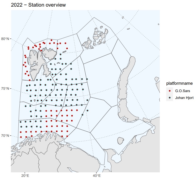
The 19-th joint Barents Sea autumn Ecosystem Survey (BESS) was carried out in two periods. The Norwegian research vessels “G.O. Sars” and “Johan Hjort” covered NEEZ in the period 16-th August to 03-th October, providing data to stock assessment, 0-group fish abundance indices, and state and changes descriptions which is comparable with earlier survey years in NEEZ. The Russian research vessel “Vilnyus” covered REEZ in the periods 20-th to 30-th September and 22-th October to 3-rd December. Survey coordinators in 2022 were Dmitry Prozorkevich (PINRO) and Geir Odd Johansen (IMR). Exchange of Russian and Norwegian experts between each country’s respective vessels did not take place in 2022. We would like to express our sincere gratitude to all the crew and scientific personnel onboard RVs “Vilnyus”, “G.O. Sars” and “Johan Hjort” for their dedicated work, as well as all the people involved in planning and reporting of BESS 2022. This report is a summary of observations and status assessment based on the survey data. Even though the survey was not well completed, the data obtained are the main source of knowledge about the ecosystem of the Barents Sea
Survey report from the joint Norwegian/Russian Ecosystem Survey in the Barents Sea and the adjacent waters August-December 2022
Report series:
IMR-PINRO 2023-10
Published: 07.11.2023
Project No.: 14153
On request by: Havforskningsinstituttet
Research group(s):
Bentiske ressurser og prosesser
,
Marin toksikologi
,
Norsk marint datasenter (NMD)
,
Oseanografi og klima
,
Pelagisk fisk
,
Plankton
,
Økosystemprosesser
,
Bunnfisk
,
Sjøpattedyr
,
Dyphavsarter og bruskfisk
Subject:
Klima i havet,
Klimaeffekter på bestander,
Klimastatus,
Plastsøppel i havet,
Radioaktiv forurensning i havet ,
Planteplankton,
Krill – Nordlig krill,
Raudåte,
Lodde – Barentshavet,
Norsk vårgytende sild,
Polartorsk,
Sei – nordaustarktisk,
Torsk – nordøstarktisk (skrei),
Hyse,
Uerfamilien,
Steinbit,
Kongekrabbe,
Reke – Barentshavet,
Snøkrabbe,
Blåhval,
Finnhval,
Knølhval,
Vågehval,
Spermhval,
Spekkhogger,
Nise
Program:
Barentshavet og Polhavet
Approved by:
Research Director(s):
Geir Huse
Program leader(s):
Maria Fossheim
External:
Oleg Bulatov (VNIRO)
Norsk sammendrag
Summary
1 - BACKGROUND
The aim of the joint Norwegian/Russian ecosystem survey in the Barents Sea and adjacent waters, August-October (BESS) is to monitor the status and changes in the Barents Sea ecosystem and provide data to support stock advice and research. The survey has since 2004 been conducted annually in the autumn, as a collaboration between the IMR in Norway and the Polar Branch of VNIRO (PINRO) in Russia. The general survey plan and tasks are usually agreed at the annual PINRO-IMR Meeting in March, but in 2022, due to external factors making physical meetings between Norwegian and Russian researchers difficult, it was agreed by correspondence. Ship routes and other technical details was agreed on by correspondence between the survey coordinators. Survey coordinators in 2022 was Dmitry Prozorkevich (PINRO) and Geir Odd Johansen (IMR). Exchange of Russian and Norwegian experts between each country’s respective vessels did not take place in 2022.
The 19-th joint Barents Sea autumn Ecosystem Survey (BESS) was carried out in two periods. The Norwegian research vessels “G.O. Sars” and “Johan Hjort” covered NEEZ in the period 16-th August to 03-th October. The Russian research vessel “Vilnyus” covered REEZ in the periods 20-th to 30-th September and 22-th October to 3-rd December.
The scientists and technicians taking part in the survey onboard the research vessels are listed in Table 1 below.
BESS 2022 was conducted during challenging times for joint survey activity and subsequent reporting of the results. Although the survey in 2022 was unsuccessful with respect to coverage in space and time, it was decided to join all the data and present them in this Joint Report for the sake of continuity, history, and to secure scientific knowledge. We would like to express our sincere gratitude to all the crew and scientific personnel onboard RVs “Vilnyus”, “G.O. Sars”, and “Johan Hjort” for their dedicated work, as well as all the people involved in planning and reporting of BESS 2022. This report is a summary of the observations and status assessments based on the survey data. The data obtained in the survey are the main source of knowledge about the ecosystem of the Barents Sea.
| Research vessel | Participants |
|---|---|
| ”Vilnyus” | (20-30.09, 22.10-03.12) |
| Pavel Krivosheya (Cruise leader, pelagic fish), Alexey Amelkin (demersal fish), Natalia Pankova (pelagic fish), Yury Kalashnikov (pelagic fish), Maxim Rybakov (demersal fish), Serafim Bryzgalov (demersal fish), Michael Nosov (instrumentation), Sergey Harlin (Instrumentation), Maksim Gubanishchev (hydrologist), Alexey Kanishchev (hydrologist), Roman Klepikovsky (sea birds and mammals), Marina Kalashnikova (parasitologist) (20-30.09.2022), Alexander Benzik (plankton, benthos), Alexandra Kudryashova (benthos). | |
| ”G.O. Sars” | Part 1 (16.08-30.08) |
| Irene Huse (Cruise leader), Penny Lee Liebig (benthos), Amalie Valde Berge (demersal fish), Hege Haraldsen (demersal fish), Lea Marie Hellenbrecht (pelagic fish), Frøydis Tousgaard Rist (pelagic fish), Jon Rønning (plankton), Anne Kari Sveistrup (benthos), Celina Eriksson Bjånes (demersal fish), Erlend Langhelle (demersal fish), Thomas André Sivertsen (sea mammals), Lars Kleivane (sea mammals), Jörn Patrick Meyer (instrumentation), Egil Frøyen (instrumentation), Monica Martinussen (plankton), Gary Elton (sea birds), Njord Svendsen (Crono - journalist). | |
| ”G.O. Sars” | Part 2 (30.08-13.9) |
| Harald Gjøsæter (Cruise leader), Penny Lee Liebig (benthos), Anne Kari Sveistrup benthos), Celina Eriksson Bjånes (demersal fish), Erlend Langhelle (demersal fish), Thomas André Sivertsen (sea mammals), Lars Kleivane (sea mammals), Jörn Patrick Meyer (instrumentation), Egil Frøyen (instrumentation), Monica Martinussen (plankton), Irene Huse (demersal fish), Eirik Odland (demersal fish), Stine Karlson (pelagic fish), Justine Diaz (pelagic fish), Hege Skaar (plankton), Gary Elton (sea birds). | |
| ”Johan Hjort” | Part 1 (18.08-12.09) |
| Tore Johannessen (Cruise leader), Mette Strand (benthos), Grethe Thorsheim (demersal fish), Sigmund Grønnevik (demersal fish), Runar Smestad (demersal fish), Anne Sæverud (demersal fish), Jan Frode Wilhelmsen (instrumentation), Hege Rognaldsen (instrumentation), Jessica Anne Hough (pelagic fish), Erling Boge (pelagic fish), Eli Gustad (plankton), Gaston Ezequiel Aguirre (plankton), Guri Nesje (chemical contaminants), Sonnich Meier (chemical contaminants), Andrey Voronkov (benthos), Yasmin Hunt (sea mammals), George McCallum (sea mammals), Jon Ford (sea birds). | |
| ”Johan Hjort” | Part 2 (12.09-06.10) |
| Georg Skaret (Cruise leader), Andrey Voronkov (benthos), Yasmin Hunt (sea mammals), George McCallum (sea mammals), Felicia Keulder-Stenevik (benthos), Hildegunn Mjanger (demersal fish), Vidar Fauskanger (demersal fish), Amalie Valde Berge (demersal fish), John Nesheim (instrumentation), Magnar Mjanger (instrumentation), Eilert Hermansen (pelagic fish), Timo Meissner (pelagic fish), Tommy Gorm-Hansen Tøsdal (pelagic fish), Terje Berge (plankton), Jane Strømstad Møgster (plankton), Jon Ford (sea birds), Sonnich Meier (chemical contaminants). |
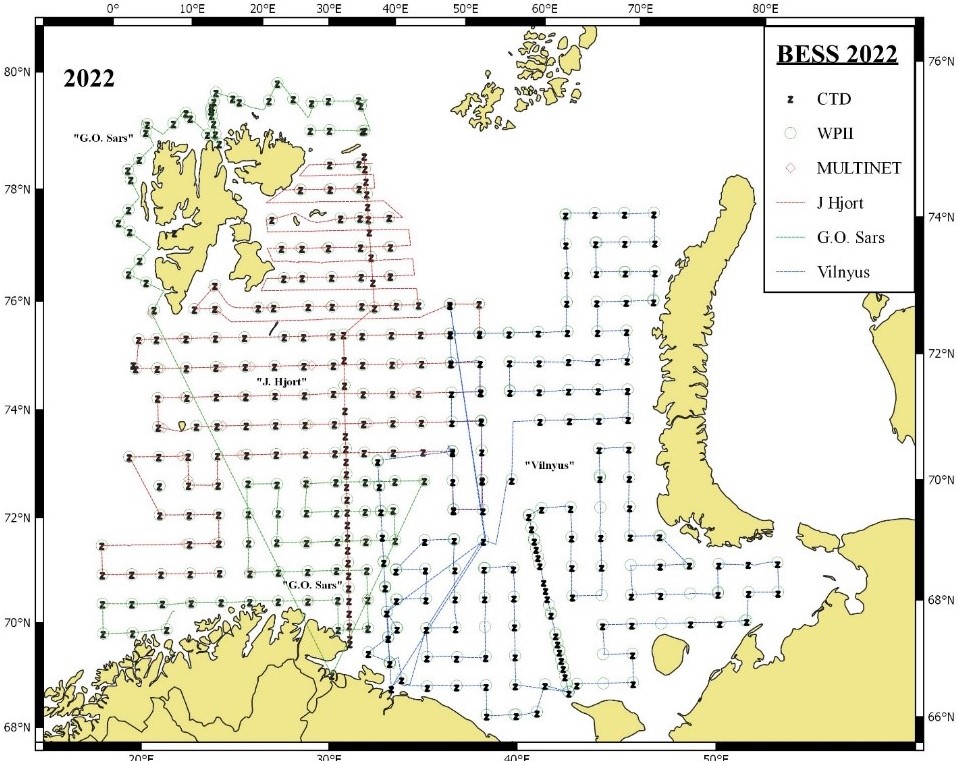
2 - SURVEY EXECUTION 2022
BESS aims at covering the entire the Barents Sea progressing from south to north. Ecosystem stations are distributed in a 35×35 nautical mile regular grid, and the ship tracks follow this design. Exceptions are the area around Svalbard (Spitsbergen), where the tracks follow a zig-zag design with additional depth stratified bottom trawl hauls for demersal fish survey indices estimation along the tracks. There are also additional acoustic transects for the capelin stock size estimation east of Svalbard (Spitsbergen).
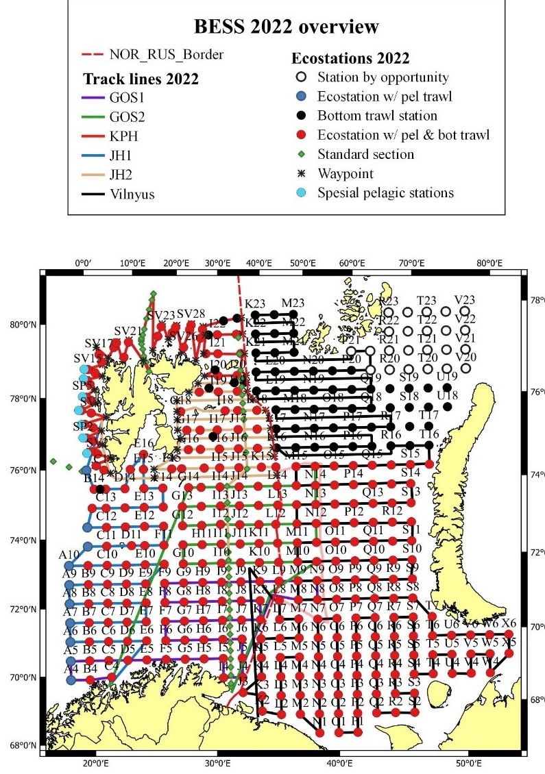
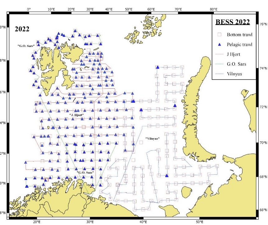
The planned vessel tracks for BESS 2022 are given in figure 2.1, but the survey was not executed according to this plan. The Russian RV “Vilnyus” covered the eastern and south-eastern of the Barents Sea within the REEZ and Loophole (bottom trawls) but missed coverage in parts of the central REEZ and in the north. Norwegian RVs covered the western part of the Barents Sea and an area around Svalbard (Spitsbergen) within the NEEZ, but the planned vessel RV “Kronprins Haakon” did not take part in the survey due to a difficult economic situation. As a result of this, RV “G.O. Sars” had to cover the southern and south-eastern part of NEEZ, and additionally the area west and north of Svalbard (Spitsbergen) to compensate for the absence of RV “Kronprins Haakon”. RV “Johan Hjort” covered the central-western part of this area and the Loophole (pelagic trawls), as well as the capelin area east of Svalbard. In addition to standard sampling at BESS, the standard oceanography sections “Vardø Nord extended” and the “Hinlopen”, were sampled in the Norwegian survey area, and the standard sections “Kola” and “Kanin” in the Russian survey area (Fig. 2.3). The realized research vessel tracks with sampling for the BESS 2022 are shown in Figure 2.2 and 2.3. Summarized, the exceptions to the planned spatial coverage were lack of coverage in the north-eastern part of the Barents Sea, thin coverage around of Svalbard (Spitsbergen), and in a central part of REEZ.
The planned time schedule for BESS 2022 was 152 consecutive days, resulting in 134 planned effective vessel days (time between first and last sample in the vessel logs). The difference between these two is as expected, as the vessels need time to prepare before sampling (e.g. testing of sampling gear and calibration), crew and personnel changes, and sail back and forth between survey area and ports related to these changes and at the end of the survey. BESS 2022 was not conducted according to the planned time schedule. Cancellation of R/V Kronprins Haakon after the cruise had started, reduced the planned effective days further to 121. Further, due to external factors, Russian vessel “Vilnius” had not received the ordered engine parts in time, resulting in delayed start of the survey part in REEZ. In addition, for various unfortunate reasons, the ship vessel to return to port several times. In total, this caused late and reduced area coverage, cancelled standard pelagic sampling in the eastern Barents Sea, and decreased number of trawl hauls in northwestern Barents Sea.
The total progression of the survey in time and space in 2022 can be characterized as being of low quality (Figure 2.4).
The consequences of the insufficient coverage in space and time of BESS 2022 is that the main ecosystem components were not well monitored. Data to stock assessment, 0-group fish abundance indices, and state and change descriptions is comparable with earlier survey years in NEEZ only. This has severe consequences for the data quality related to several ecosystem components, including assessment of several commercial species, and conclusions made based on these data must be viewed as highly uncertain.
2.1 Sampling methods
Some adjustments of sampling gear were done in 2022 compared to 2021. At Norwegian vessels, the rigging of the 0- group trawl (Harstad trawl) was changed by using new lining. Special net for juvenile shrimp were taken out as standard at bottom trawl hauls. Manta trawl was included as standard equipment for monitoring microplastic at BESS from 2021 and microplastic samples were also collected in 2022. A new length stratified individual sampling of haddock was tested out in 2022 measuring. Monitoring of phytoplankton with algae nets and CTD water samples was removed from the sampling plan at regular stations in 2022 and will in the future only be taken at the hydrographic standard sections Vardø Nord extended and Hinlopen. Some minor changes in the sampling procedures for snow crab was also introduced.
The survey sampling manuals can be obtained by contacting the survey coordinators. These manuals include methodological and technical descriptions of equipment, the trawling and capture procedures by the sampling tools, sampling and registration of the catch in the lab, and the methods that are used for calculating the abundance and biomass of the biota.
2.2 Special investigations
BESS is a useful platform for conducting additional studies in the Barents Sea. These studies can be testing of new methodology, sampling of data additional to the standard monitoring, or sampling of other types of data. It is imperative that the special investigations do not influence the standard monitoring activities at the survey. The special investigations vary from year to year, and below is a list of special investigation conducted on Russian Norwegian vessels at BESS 2022, with contact persons.
2.2.1 Annual monitoring of pollution levels
In 2022 PINRO continued the annual monitoring of pollution levels in the Barents Sea in accordance with a national program. Samples of seawater, sediments, fish and invertebrates was collected and analysed for persistent organic pollutants (POPs) (e.g. PCBs, DDTs, HCHs, HCB) and heavy metals (e.g. lead, cadmium, mercury) and arsenic. The samples were collected at RV "Vilnyus" during BESS in the southern and eastern parts of the Barents Sea. The results from chemical analyses will be reported in 2023.
Contact: Mikhail Novikov, PINRO (mnovik@pinro.ru)
2.2.2 Collection of samples for biochemical studies
Frozen samples of commercial and non-commercial fish and invertebrates were collected for biochemical studies (ratio of body parts, chemical composition of nutrients, molecular weight of muscle proteins, amino acids and lipid fractions composition) in accordance with a research program. Samples were frozen at a temperature not higher than minus 18° C immediately after catching before rigor mortis.
Contact: Kira Rysakova, PINRO (rysakova@pinro.ru)
2.2.3 Fish pathology research
PINRO undertakes yearly investigations of fish and crabs diseases and parasites in the Barents Sea (mainly in REEZ). This investigation was started by PINRO in 1999. The main purpose of the pathology research is annual estimation of epizootic state of commercial fish and crabs species. The observations are entered into a database on pathology named “Pathology of fish in the seas of the Arctic ocean and the North-East Atlantic”.
Contact: Tatyana Karaseva, PINRO (karaseva@pinro.ru)
Link to more information:
https://www.amazon.com/Barents-Sea-Ecosystem-Management-Cooperation/dp/8251925452 (pp. 743-749)
2.2.4 Parasitological study
The purpose of this study is to monitor the infestation of commercial fish species in the Barents Sea with helminths that are hazardous to human health. 200 specimens of six fish species were studied in order to identify of such helminths. Statistical processing of parasitological data consisted in determination of three indicators of the degree of parasite infestation: prevalence – the proportion (%) of fish infested with a parasite of this species of the number of examined fish; abundance – the number of parasites of this species per one examined fish; confidence interval (CI) – the interval that covers the parameter of the prevalence with a designated confidence level. Helminths of two species that are hazardous to human health have been identified (larvae of nematodes Anisakis simplex and Pseudoterranova spp.). The first of them are mostly found in cod, haddock and long rough dab. Capelin and Arctic cod are infested with them to a lesser extent (Tables 2.2.4.1; 2.2.4.2).
Table 2.2.4.1. Indicators of the total infestation of fish with larvae of the nematode Anisakis simplex.
| Fish species |
Number of examined fish, specimens |
Average length (min-max), cm |
Infestation rates Prevalence (CI), % |
Abundance, specimens |
| Cod | 25 | 47.1 (27.0-72.0) | 92.0 (78.1-99.2) | 11,2 |
| Haddock | 25 | 34.8 (21.0-51.0) | 96.0 (84.7-100) | 25,7 |
| European plaice | 25 | 39.3 (33.0-54.0) | 12.0 (2.3-27.7) | 0,1 |
| Long rough dab | 25 | 31.0 (21.0-43.0) | 76.0 (57.3-90.6) | 6,2 |
| Capelin | 25 | 15.7 (13.5-18.0) | 40.0 (27.7-59.9) | 0,4 |
| Arctic cod | 75 | 18.0 (11.0-27.5) | 52.0 (40.5-63.4) | 0,9 |
Table 2.2.4.2. Indicators of the total infestation of fish with larvae of the nematode Pseudoterranova spp.
| Fish species |
Number of examined fish, specimens |
Average length (min-max), cm |
Infestation rates Prevalence (CI), % |
Abundance, specimens |
| Long rough dab | 25 | 31.0 (21.0-43.0) | 4.0 (0.0-15.3) | 0,04 |
The obtained data indicate a consistent high level of invasion of most bottom fish species with the nematode A. simplex.
Contact: Yuri Bakay, PINRO (bakay@pinro.ru)
3 - DATA MANAGEMENT
3.1 Databases
A wide variety of data are collected during the ecosystem surveys. All data collected during the BESS are quality controlled and verified by experts from IMR and PINRO during the survey. The data are stored in IMR and PINRO national databases, with different formats. However, the data are exchanged so that both institutions have access to each other’s data in their respective databases (i.e. both institutes use equal joint data).
3.2 Data application
The main aim of the BESS is to cover the whole Barents Sea ecosystem geographically and provide survey data for commercial fish and shellfish stock estimation. Stock estimation is particularly important for capelin, because capelin TAC is based on the survey result, and the Norwegian-Russian Fishery Commission determines TAC immediately after the survey. In addition, a broad spectrum of physical variables, ecosystem components and pollution are monitored and reported.
The survey data will be used by Norway and Russia for the implementation the joint or national projects. In addition, each of the side uses the survey data for participate in their international projects.
This survey report is based on joint data and contains the main results of the monitoring. The survey report is published as part of the IMR/PINRO Joint Report series and assembled into a complete pdf-report when the main components are completed. Some post-survey information not included in the written report (e.g. plankton and fish stomach samples which need longer processing time) will be published as individual parts of the report later. All reports from BESS from 2004 until the latest are available at this web site: https://imr.brage.unit.no/imr-xmlui/handle/11250/2658167. This report is published in the IMR digital report series IMR-PINRO.
3.3 Time series of distribution maps
The redesigned IMR web site for the joint Norwegian/Russian Barents Sea Ecosystem Surveys is still not finished. The maps from this report series are to be made public in this map site when ready.
4 - MARINE ENVIRONMENT
4.1 Hydrography
Text by: Alexander Trofimov and Randi Ingvaldsen
Figures by: A. Trofimov
4.1.1 Geographic variation
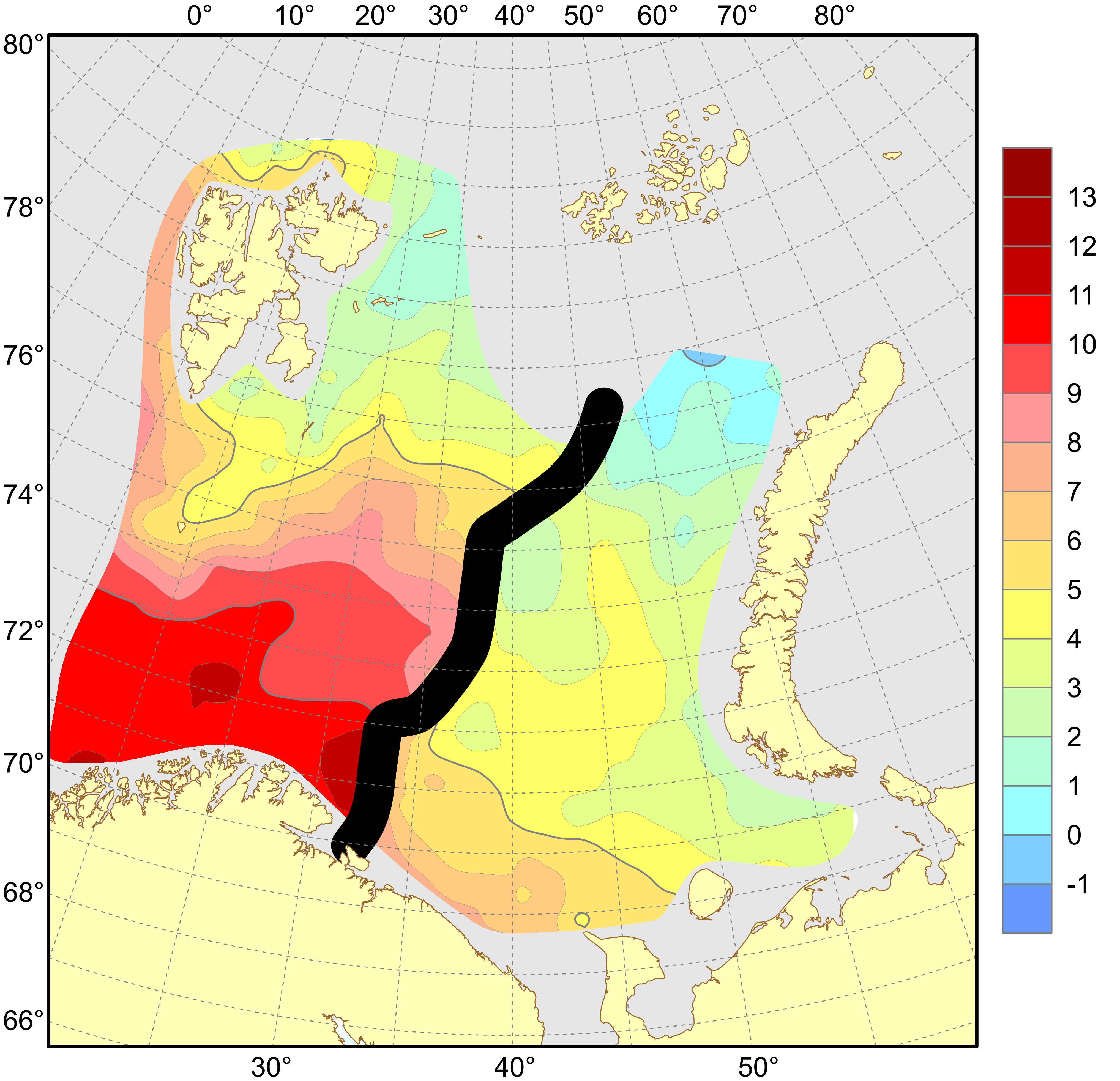
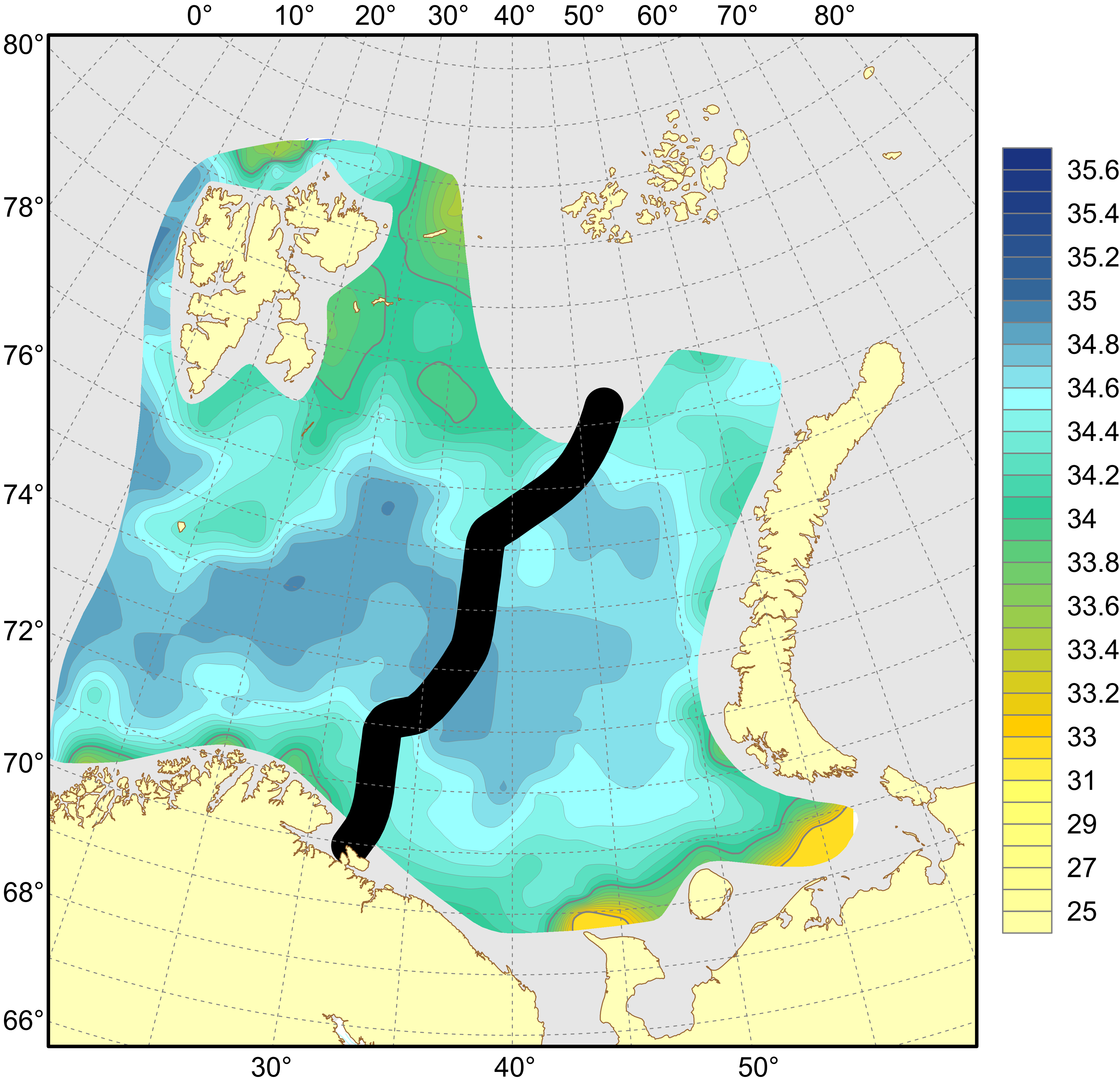
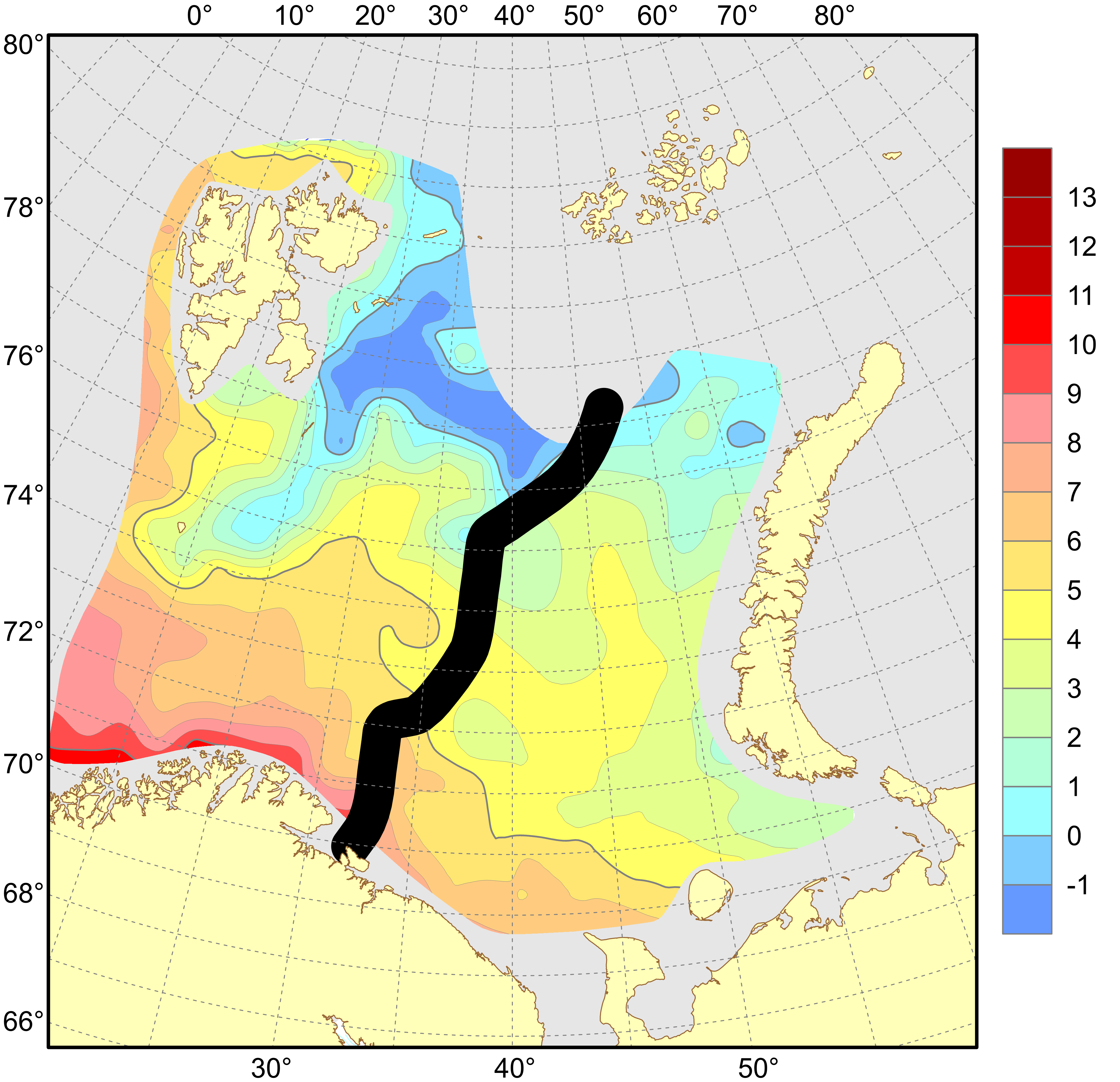
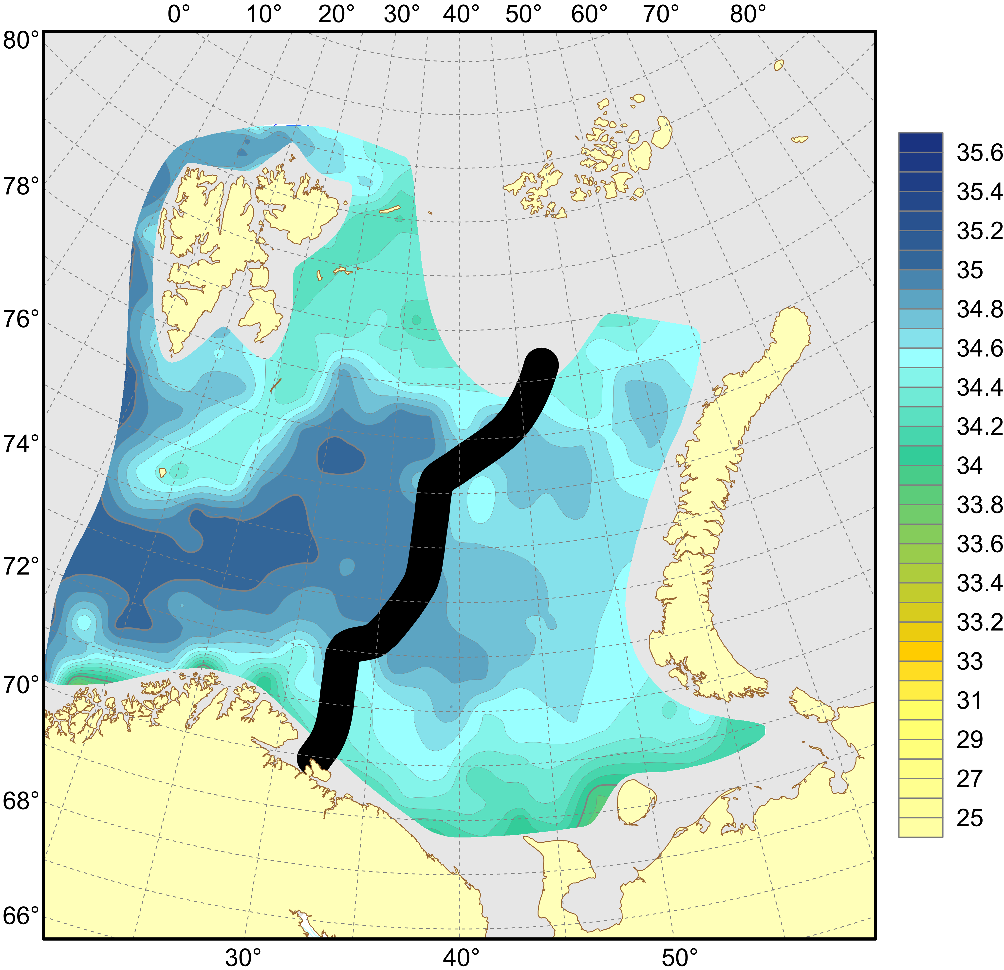
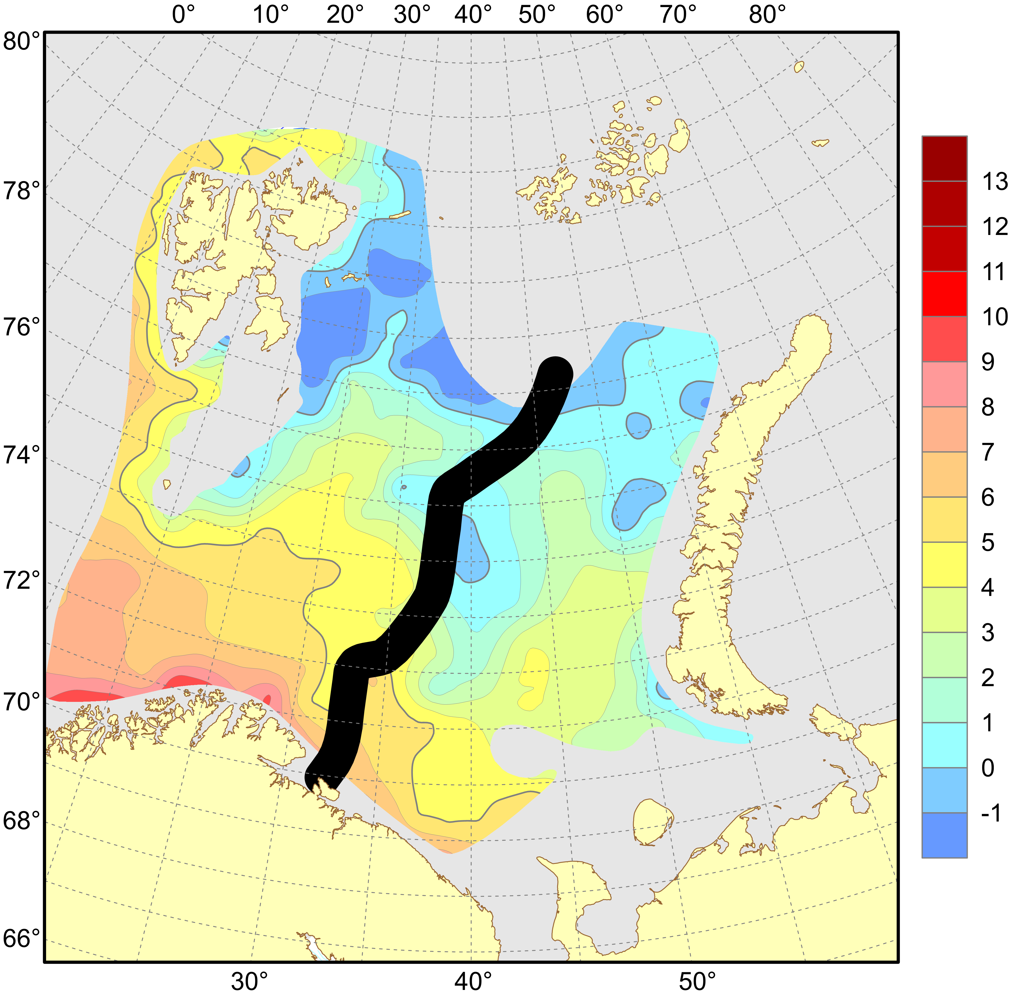
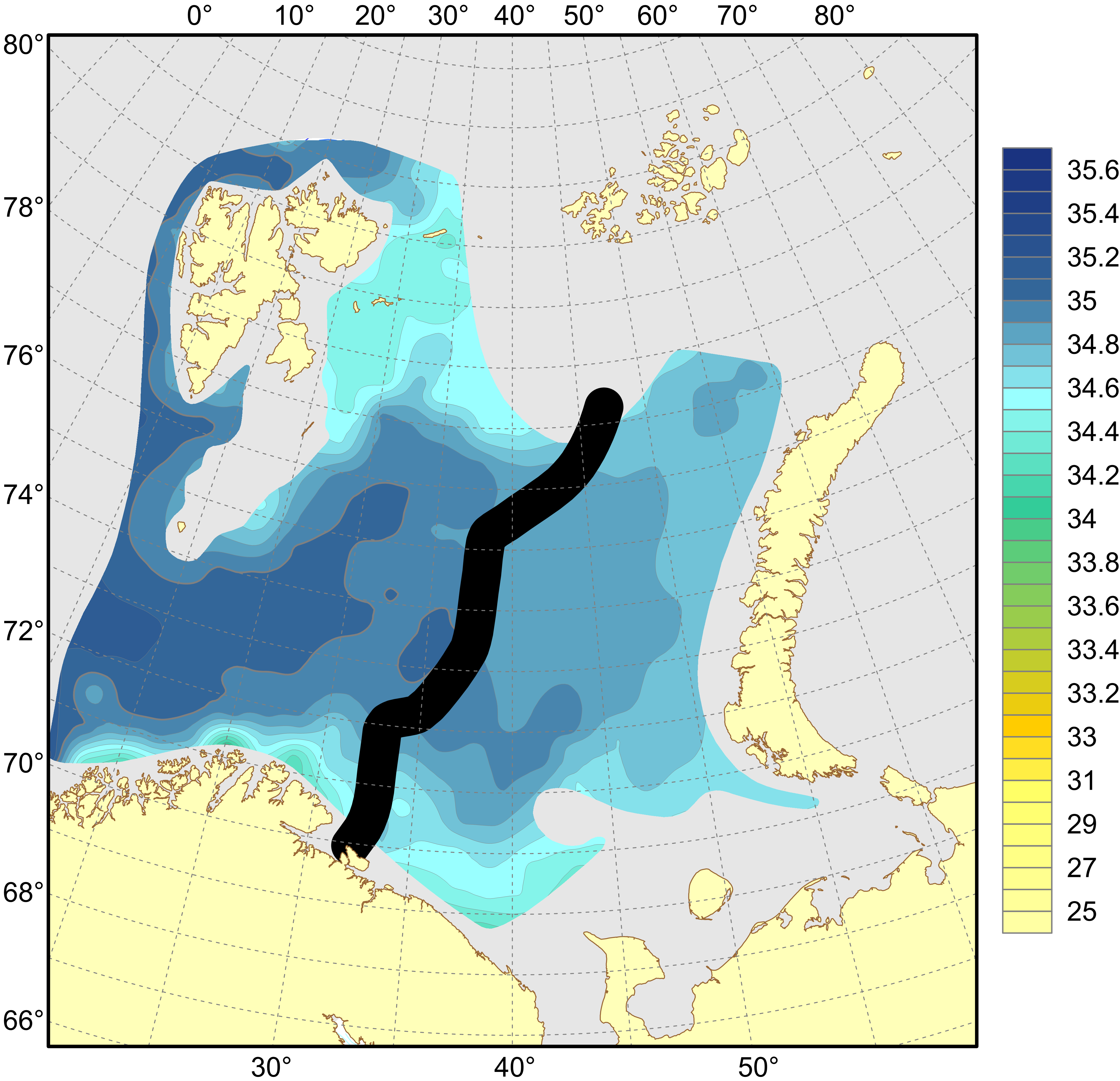
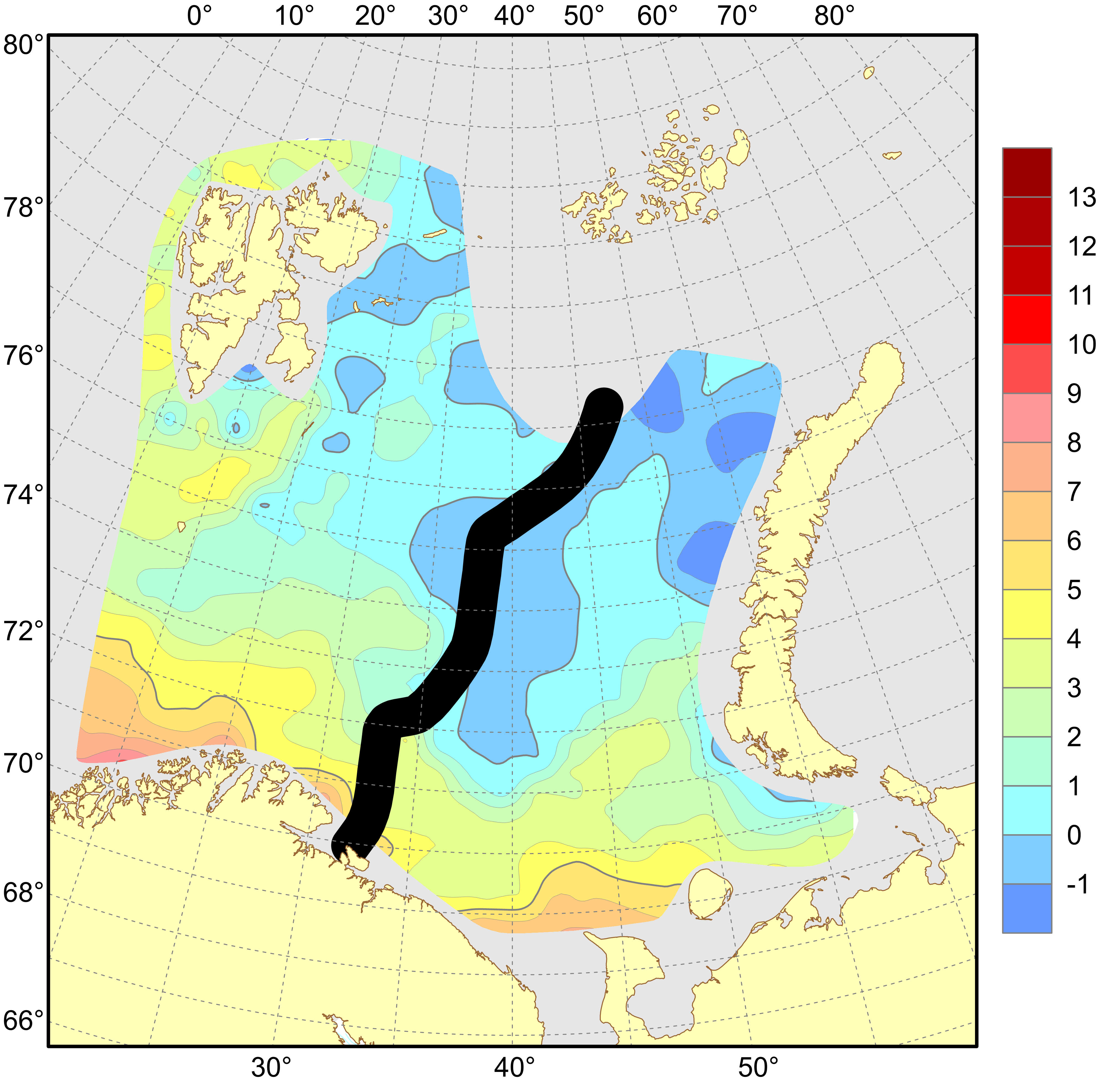
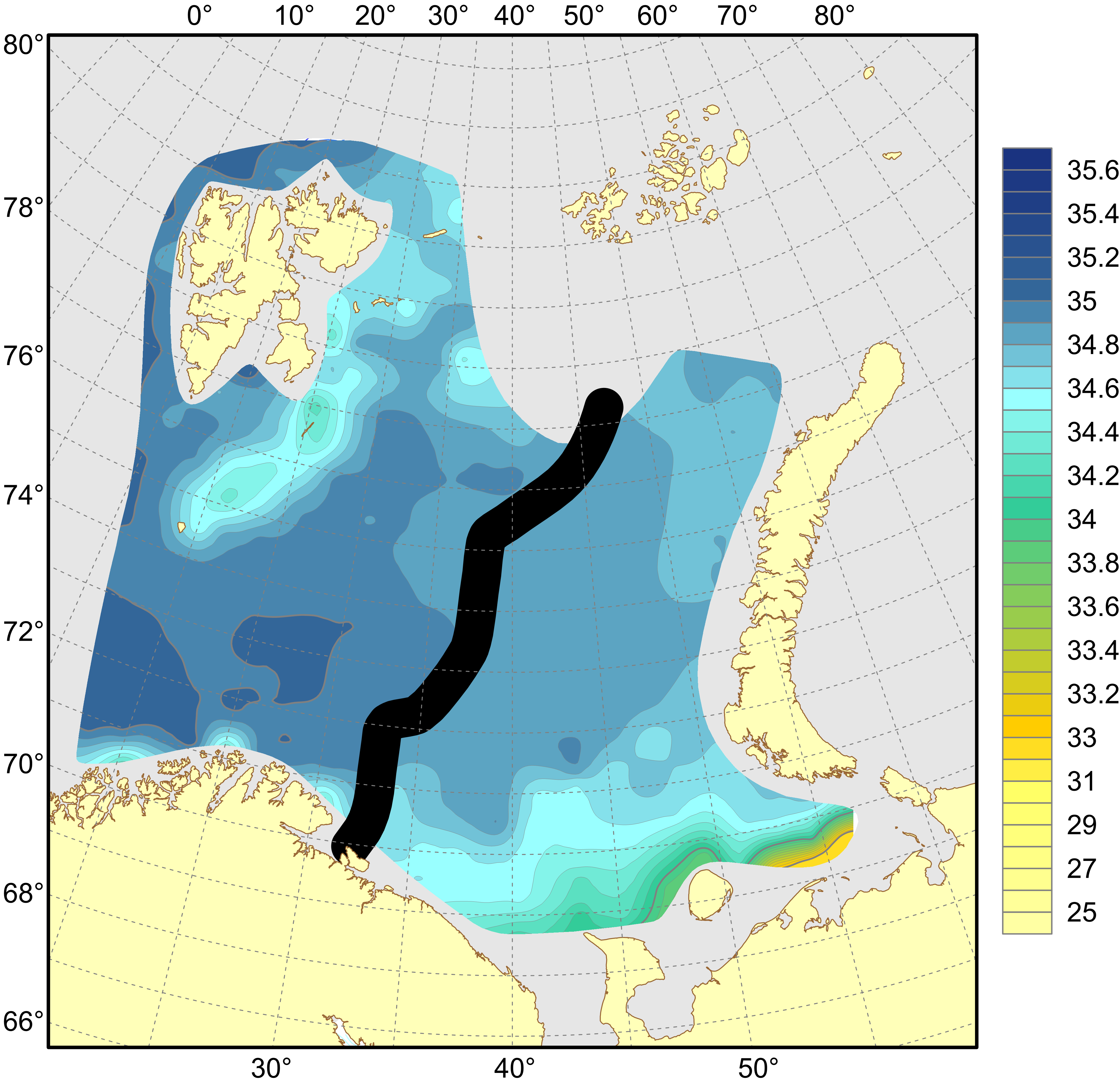
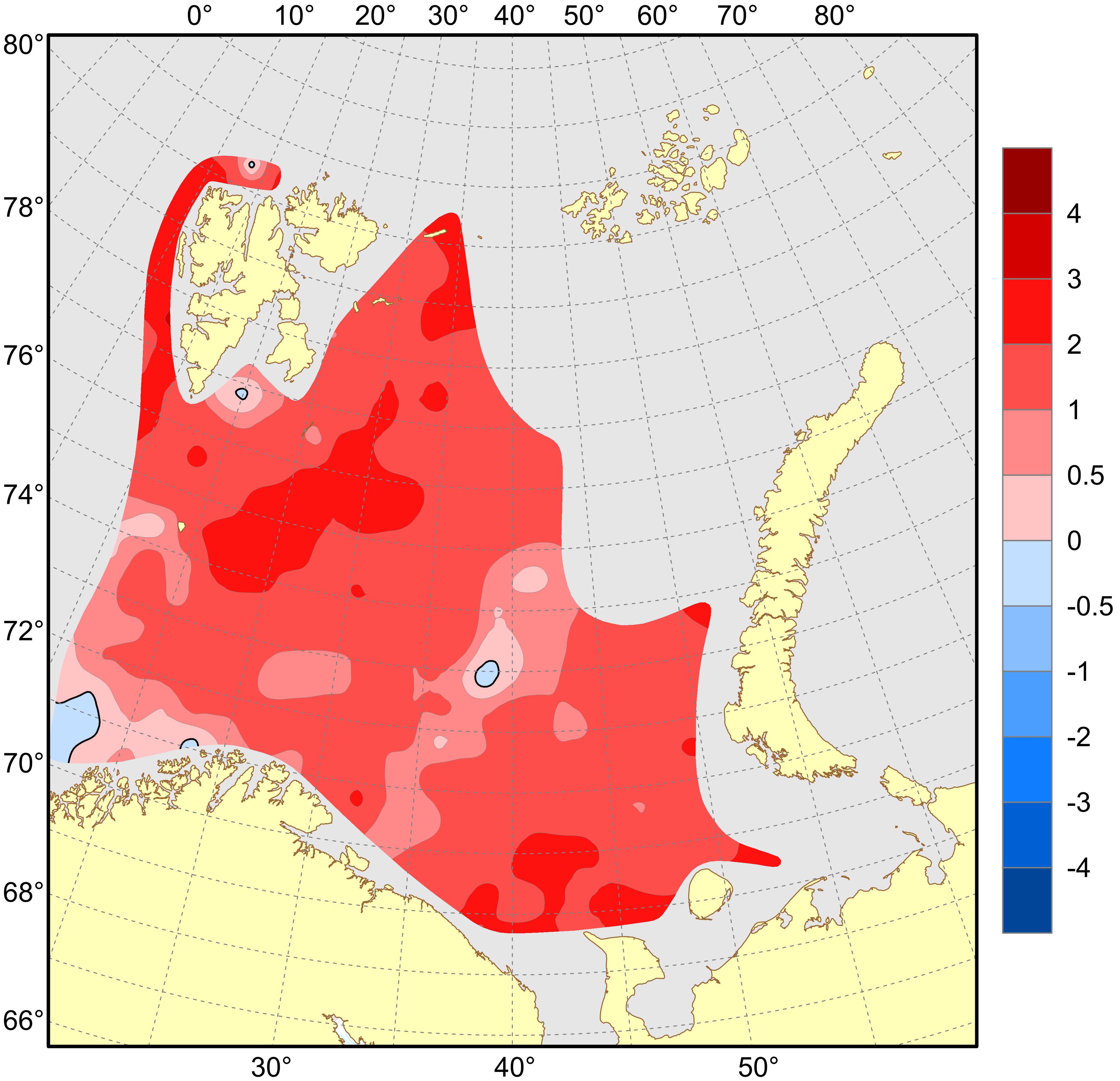
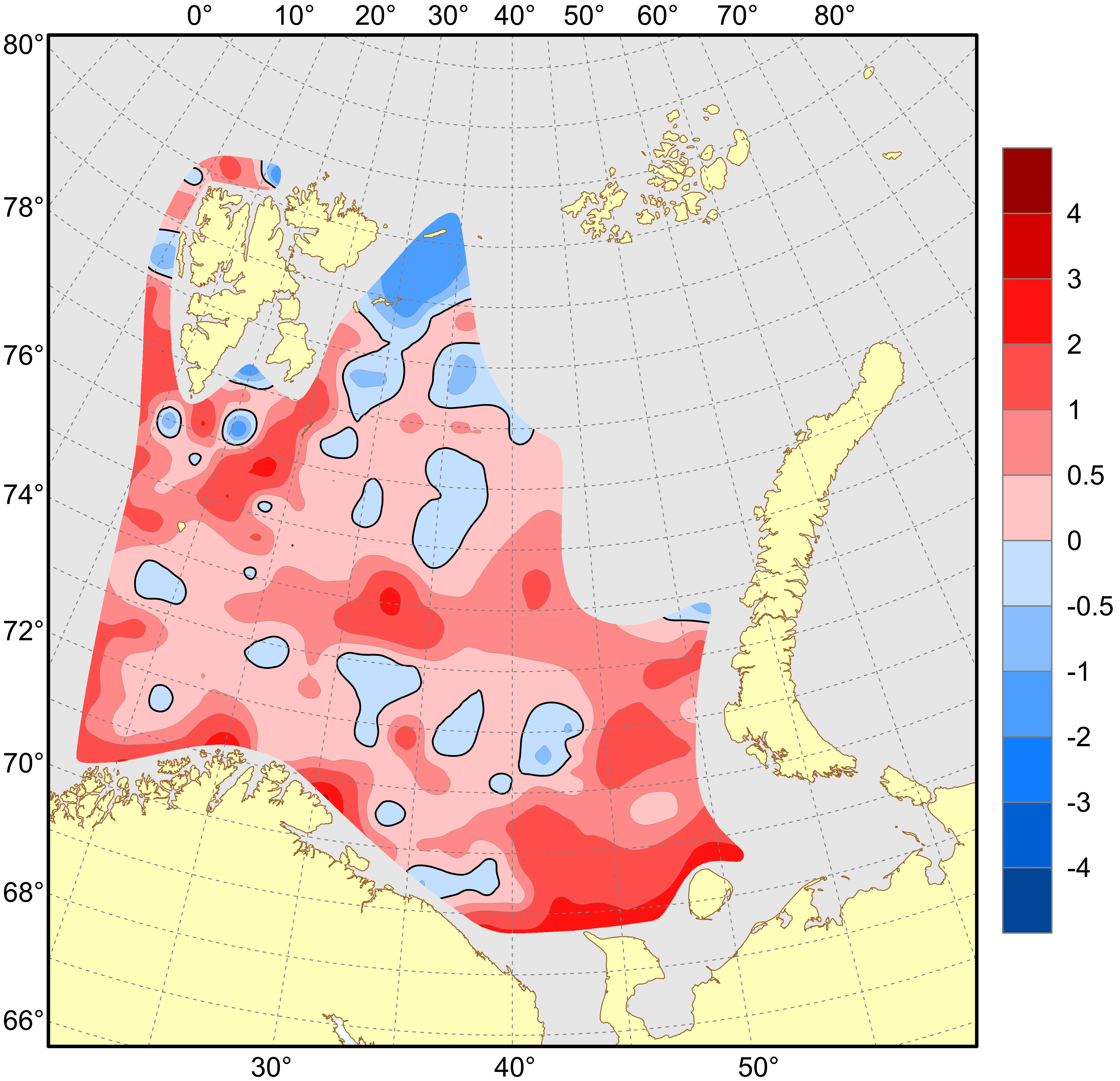
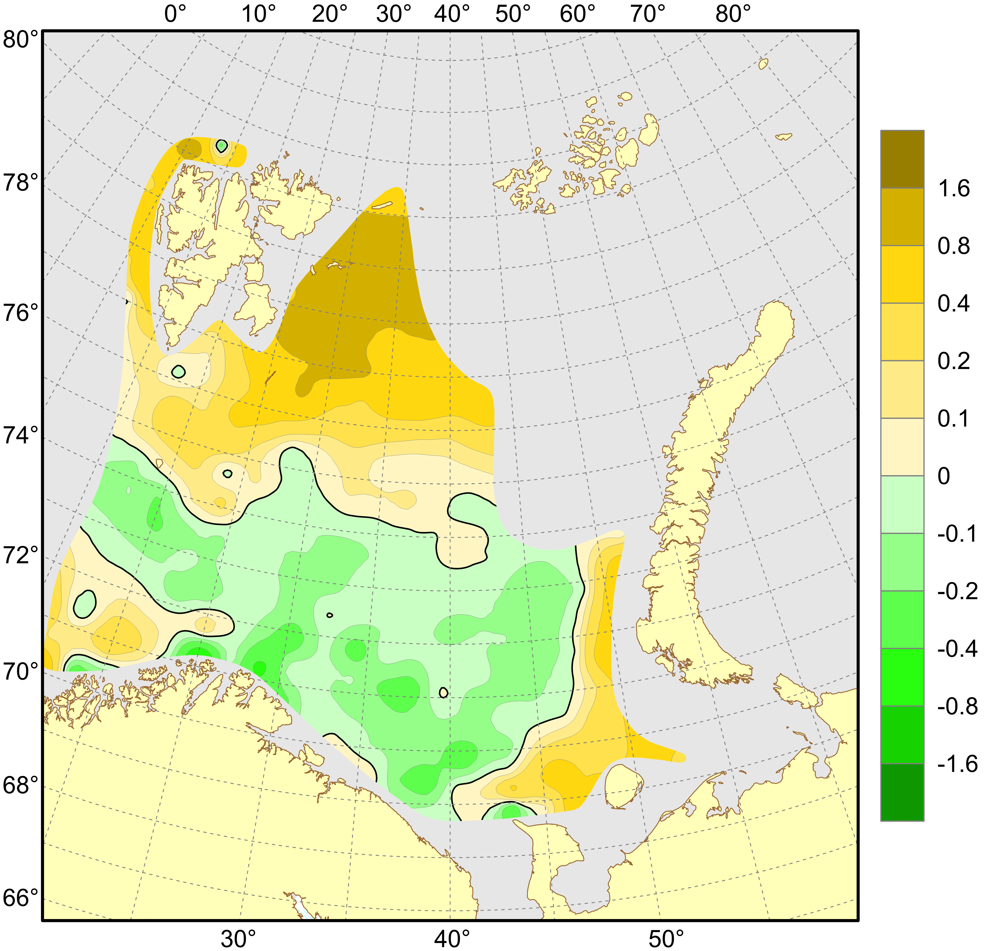
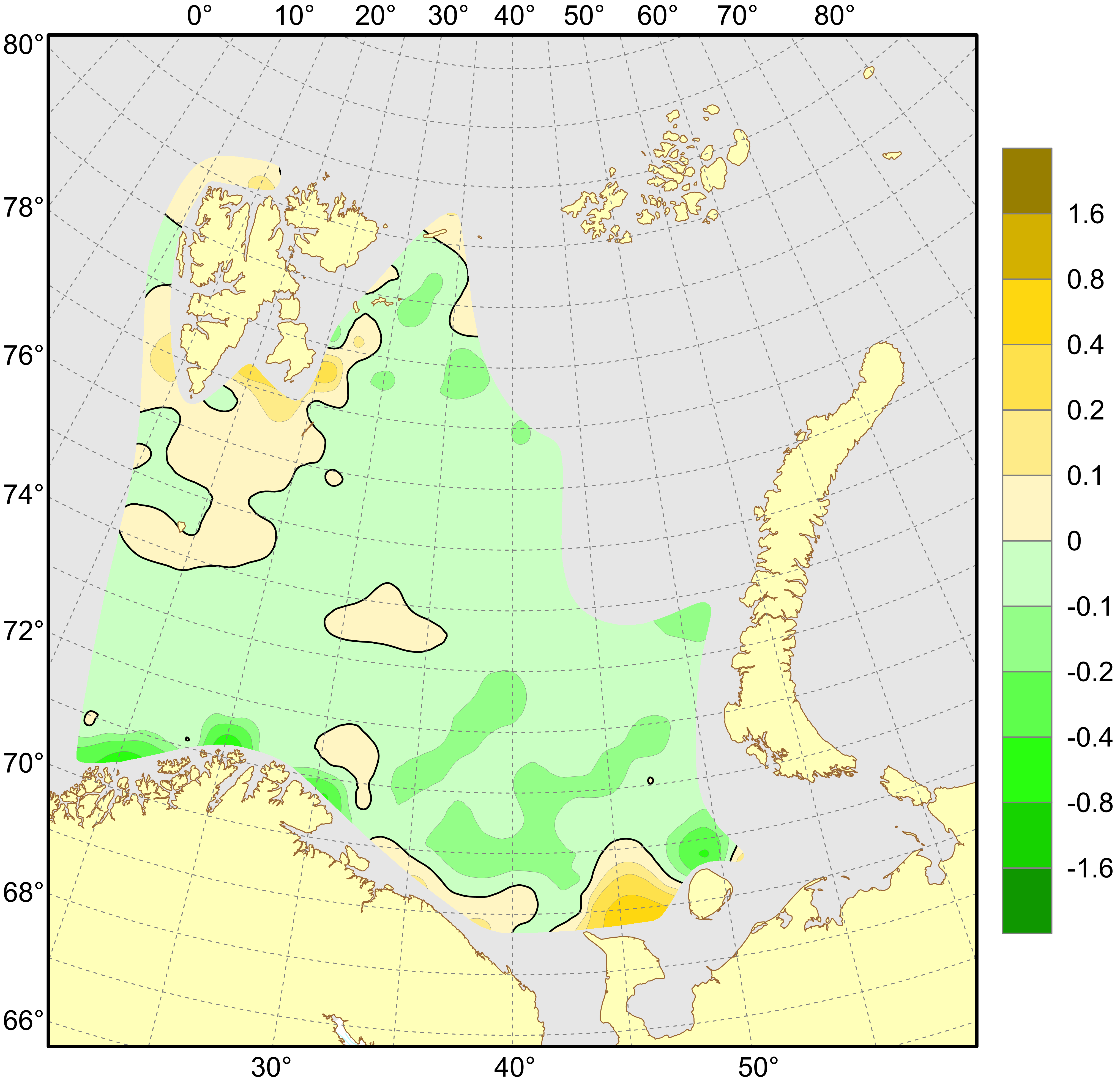
Horizontal distributions of temperature and salinity are shown for depths of 0, 50, 100 m and near the bottom in Figs 4.1.1.1–4.1.1.8, and anomalies of temperature and salinity at the surface and near the bottom are presented in Figs 4.1.1.9–4.1.1.12. The anomalies have been calculated using the long-term means for the period 1981–2010.
In autumn 2022, surface temperature was on average 1.5°C higher than the long-term mean all over the surveyed area (Fig. 4.1.1.9). Compared to 2021, the surface temperature in 2022 was much higher (by 1.2°C on average) almost all over the surveyed area (94%), with the largest positive differences (>2°C) in the western Barents Sea.
Arctic waters were mainly found, as usual, in the 50–100 m layer north of 77°N (Fig. 4.1.1.3 and 4.1.1.5). Temperatures at depths of 50 and 100 m were higher than the long-term means (on average, by 1.0 and 0.7°C respectively) in most of the surveyed area (89 and 84%), with the largest positive anomalies at 50 m depth in the southeast. Negative anomalies (about −0.3°C on average) were mostly found at 100 m depth in the northern Barents Sea. Compared to 2021, the 50 and 100 m temperatures in 2022 were higher (on average, by 0.6 and 0.5°C respectively) in two thirds of the surveyed area. Negative differences were observed in some separate areas of the Barents Sea. Small differences (both negative and positive, <0.5°C in magnitude) prevailed at 100 m depth.
Bottom temperature was in general 0.7°C above average in most of the surveyed area (83%), with the largest positive anomalies in the southeastern Barents Sea (Fig. 4.1.1.10). Negative anomalies were mainly found in the northernmost part of the sea, between the Spitsbergen and Franz Josef Land archipelagoes. In bottom waters, small temperature differences between 2022 and 2021 (both negative and positive, <0.5°C in magnitude) prevailed (~70% of the surveyed area). In autumn 2022, the area covered by bottom water with temperatures below zero was 37% in the Barents Sea (71–79°N 25–55°E) being close to those in the previous two years.
Surface salinity was on average 0.4 higher than the long-term mean in half of the surveyed area, namely in the northern, easternmost and southwesternmost Barents Sea, with the largest positive anomalies (>0.8) in the north (Fig. 4.1.1.11). Negative anomalies (–0.1 on average) were mainly observed in the southern part of the sea. In autumn 2022, surface waters were on average 0.2 fresher than in 2021 in 62% of the surveyed area; they were saltier (on average, by 0.3) in the northern and southwesternmost Barents Sea as well as in a small area west and north of Kolguev Island.
Salinity at 50 m depth was lower than average (by 0.1 on average) in most of the surveyed area (60%), with the largest negative anomalies in coastal waters in the southwestern Barents Sea. Positive anomalies were mainly observed in the northern (especially east of the Spitsbergen Archipelago) and southeasternmost parts of the sea. In autumn 2022, waters at 50 m were saltier (by 0.1 on average) than in 2021 in half of the surveyed area, with the largest positive differences over the Spitsbergen Bank and west and northwest of Kolguev Island. Significant negative differences (>0.1 in magnitude) in 50 m salinity between 2022 and 2021 were mainly observed in the south and east. At a depth of 50 m, both positive and negative anomalies and differences were larger than at 100 m. At a depth of 100 m, salinity anomalies and differences of <0.1 in magnitude occupied about 90% of the surveyed area.
Bottom salinity was slightly lower than average almost all over the surveyed area (80%), with the largest negative anomalies (>0.1 in magnitude) in some small areas in the southern Barents Sea (Fig. 4.1.1.12). Positive anomalies were mainly found south of the Spitsbergen Archipelago and west of Kolguev Island. In autumn 2022, bottom waters were a bit saltier than in 2021 in two thirds of the surveyed area, with the largest positive differences (>0.1) over the Spitsbergen Bank and west and north of Kolguev Island. As a whole, bottom salinity anomalies and differences were small (<0.1 in magnitude) almost all over the surveyed area (85 and 88% respectively).
4.1.2 Standard sections
Table 4.1.2.1 shows mean temperatures in the main parts of standard oceanographic sections of the Barents Sea, along with historical data back to 1965.
The Fugløya–Bear Island and Vardø–North Sections cover the inflow of Atlantic and Coastal water masses from the Norwegian Sea to the Barents Sea. The mean Atlantic Water (50–200 m) temperature in the inflow region to the Barents Sea, i.e., at the Fugløya–Bear Island Section, was 0.4°C higher than the long-term mean (1981–2010) and 0.3°C warmer than in 2021 (Table 4.1.2.1). The temperature in the Vardø–North Section was at the same level as in 2021 (Table 4.1.2.1).
The Kola Section covers the flow of coastal and Atlantic waters in the southern Barents Sea. In autumn 2022, the Kola Section was sampled in late October. Temperature anomalies (averaged over 50–200 m, relative to 1981–2010) were decreasing from +0.8°C in coastal waters in the inner part of the Kola Section to +0.7 and +0.4°C in Atlantic waters in the central and outer parts respectively, that was typical of warm years. The anomalies were also decreasing with depth: from +1.4 and +0.8°C (0–50 m) to +0.3°C (150–200 m) in the central and outer parts of the section. Compared to 2021, the upper 50 m layer along the Kola Section in October 2022 was 0.7–1.0°C warmer; the 50–200 m layer was 0.1–0.4°C warmer; and temperature in the 150–200 m layer was close to that in 2021.
Table 4.1.2.1. Mean water temperatures in the main parts of standard oceanographic sections in the Barents Sea and adjacent waters in August–September 1965–2022. The sections are: Kola (70º30′N – 72º30′N, 33º30′E), Kanin S (68º45′N – 70º05′N, 43º15′E), Kanin N (71º00′N – 72º00′N, 43º15′E), Vardø – North (VN, 72º15′N – 74º15′N, 31º13′E) and Fugløya – Bear Island (FBI, 71º30′N, 19º48′E – 73º30′N, 19º20′E).
|
Year |
Section and layer (depth in metres) |
||||||
|
Kola |
Kola |
Kola |
Kanin S |
Kanin N |
VN |
FBI |
|
|
0–50 |
50–200 |
0–200 |
0–bot. |
0–bot. |
50–200 |
50–200 |
|
|
1965 1966 1967 1968 1969 1970 1971 1972 1973 1974 1975 1976 1977 1978 1979 1980 1981 1982 1983 1984 1985 1986 1987 1988 1989 1990 1991 1992 1993 1994 1995 1996 1997 1998 1999 2000 2001 2002 2003 2004 2005 2006 2007 2008 2009 2010 2011 2012 2013 2014 2015 2016 2017 2018 2019 2020 2021 2022 |
6.7 6.7 7.5 6.4 6.7 7.8 7.1 8.7 7.7 8.1 7.0 8.1 6.9 6.6 6.5 7.4 6.6 7.1 8.1 7.7 7.1 7.5 6.2 7.0 8.6 8.1 7.7 7.5 7.5 7.7 7.6 7.6 7.3 8.4 7.4 7.6 6.9 8.6 7.2 9.0 8.0 8.3 8.2 6.9 7.2 7.8 7.6 8.2 8.8 8.0 8.5 8.7 7.9 8.1 7.8 8.2 7.9 - |
3.9 2.6 4.0 3.7 3.1 3.7 3.2 4.0 4.5 3.9 4.6 4.0 3.4 2.5 2.9 3.5 2.7 4.0 4.8 4.1 3.5 3.5 3.3 3.7 4.8 4.4 4.5 4.6 4.0 3.9 4.9 3.7 3.4 3.4 3.8 4.5 4.0 4.8 4.0 4.7 4.4 5.3 4.6 4.6 4.3 4.7 4.0 5.3 4.6 4.6 4.8 4.7 4.8 4.9 4.4 4.3 4.5 - |
4.6 3.6 4.9 4.4 4.0 4.7 4.2 5.2 5.3 4.9 5.2 5.0 4.3 3.6 3.8 4.5 3.7 4.8 5.6 5.0 4.4 4.5 4.0 4.5 5.8 5.3 5.3 5.3 4.9 4.8 5.6 4.7 4.4 4.7 4.7 5.3 4.7 5.8 4.8 5.7 5.3 6.1 5.5 5.2 5.0 5.5 4.9 6.0 5.6 5.4 5.7 5.8 5.6 5.7 5.2 5.3 5.3 - |
4.6 1.9 6.1 4.7 2.6 4.0 4.0 5.1 5.7 4.6 5.6 4.9 4.1 2.4 2.0 3.3 2.7 4.5 5.1 4.5 3.4 3.9 2.7 3.8 6.5 5.0 4.8 5.0 4.4 4.6 5.9 5.2 4.2 2.1 3.8 5.8 5.6 4.0 4.2 5.0 5.2 6.1 4.9 4.2 - 4.9 5.0 6.2 5.5 4.5 6.1 - - - 5.5 - 6.0 - |
3.7 2.2 3.4 2.8 2.0 3.3 3.2 4.1 4.2 3.5 3.6 4.4 2.9 1.7 1.4 3.0 2.2 2.8 4.2 3.6 3.4 3.2 2.5 2.9 4.3 3.9 4.2 4.0 3.4 3.4 4.3 2.9 2.8 1.9 3.1 4.1 4.0 3.7 3.3 4.2 3.8 4.5 4.3 4.0 4.3 4.5 3.8 5.2 4.6 4.1 4.6 5.5 - - 4.1 - 4.3 - |
3.8 3.2 4.4 3.4 3.8 4.1 3.8 4.6 4.9 4.3 4.5 4.4 3.6 3.2 3.6 3.7 3.4 4.1 4.8 4.2 3.7 3.8 3.5 3.8 5.1 5.0 4.8 4.6 4.2 4.8 4.6 3.7 4.0 3.9 4.8 4.2 4.2 4.6 4.7 4.8 5.0 5.3 4.9 4.7 5.2 - 5.1 5.7 4.9 5.2 5.5 5.1 5.2 - 4.7 5.1 5.0 5.0 |
5.2 5.3 6.3 5.0 6.3 5.6 5.6 6.1 5.7 5.8 5.7 5.8 4.9 4.9 4.7 5.5 5.3 6.0 6.1 5.7 5.6 5.5 5.1 5.7 6.2 6.3 6.2 6.1 5.8 5.9 6.1 5.7 5.4 5.8 6.1 5.8 5.9 6.5 6.2 6.4 6.2 6.9 6.5 6.4 6.4 6.2 6.4 6.4 6.3 6.1 6.6 6.5 6.4 6.0 5.9 6.2 6.1 6.4 |
|
Average 1981–2010 |
7.6 |
4.2 |
5.0 |
4.6 |
3.6 |
4.4 |
6.0 |
4.2 Antropogenic pollution
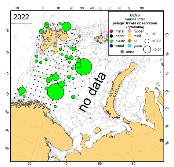
4.2.1 Marine litter
Text by: T. Prokhorova, B. E. Grøsvik, P. Krivosheya
Figures by: P. Krivosheya
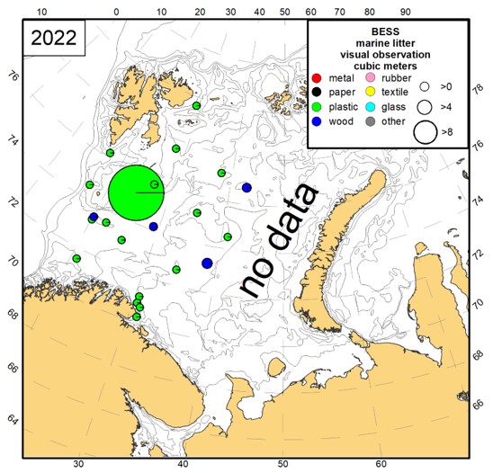
Anthropogenic litter floating at the surface was observed from the Norwegian vessels only. Plastics dominated among anthropogenic pollutants on the water surface (81.5 % of observations) (Fig. 4.2.1.1). The maximum surface observation of plastic litter was 12 m3, and it was a part of fishery trawl. The average surface observation of plastic was 0.005 m3 (except the single maximum catch of 12 m3). Due to currents, recorded debris could be dumped directly in some areas and transported from other areas. Wood was recorded in 18.5 % of the observations. The maximum surface observation of wood was 0.6 m3, while the average was 0.4 m3. Wood was presented by logs and pallets. Strictly, wood is not a pollution item, but we have presented wood in this report traditionally as litter.
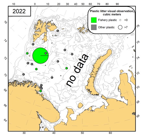
Fishery related litter was recorded in 22.7 % of plastic litter observations at the surface (Fig. 4.2.1.2). Fishery related litter was represented by floats/buoys (OSPAR code 37) and pieces of net (OSPAR code 116). Fishery plastic both maximum and average observations (12 m3 and 0.01 m3 (except the single maximum catch of 12 m3) was larger than non-fishery plastic (0.03 m3 and 0.003 m3).
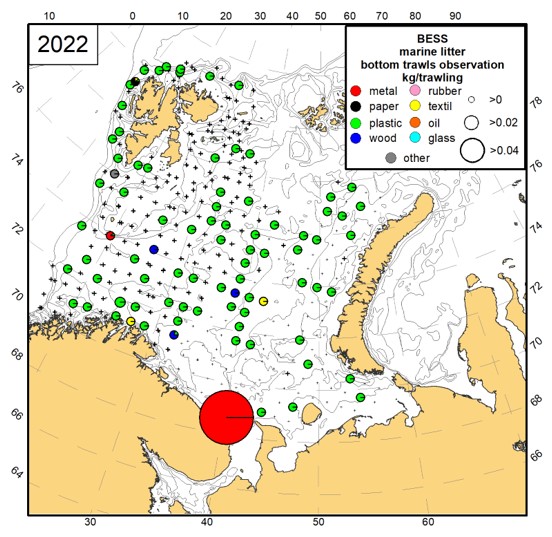
Anthropogenic litter collected in bottom trawls in 2022 was observed onboard all Norwegian vessels and Russian vessel “Vilnyus”, in pelagic trawls – onboard the Norwegian vessels only.
Anthropogenic litter was observed in 17.6 % of pelagic trawl stations (Fig. 4.2.1.3). Only plastic was observed in pelagic trawls with anthropogenic litter in 2022. The minimum catch of plastic by pelagic trawl was 0.0004 kg per n.mile, the maximum catch was 0.04 kg per n.mile, with the average of 0.005 kg per n.mile. Considering the low catchability by pelagic trawl for low-density polymers, the total amount of this matter in the Barents Sea could be much higher.
Litter was observed in 34.9 % of the bottom trawl stations in 2022 (Fig. 4.2.1.4), and it is higher than in 2021 (28.1 % of the bottom trawl stations). The minimum catch of litter by bottom trawl was 0.00002 kg per n.mile. the maximum catch was 602.4 kg per n.mile, with the average of 0.360 kg per n.mile (except the single maximum catch of 500 kg).
Plastic dominated the litter content from the bottom trawls as usual (78.6 % of stations with observed litter). The catch of plastic litter in bottom trawls was from 0.00002 kg per n.mile to 26.5 kg per n.mile with average of 0.4 kg per n.mile. Wood, textile and metal were observed sporadically among the bottom trawl catches.
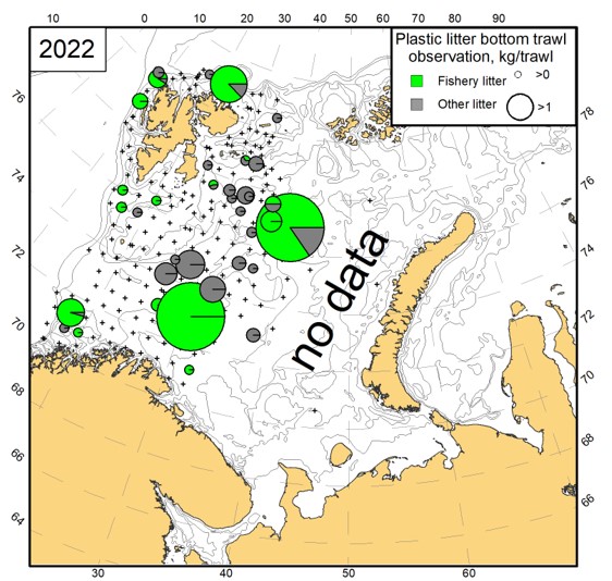
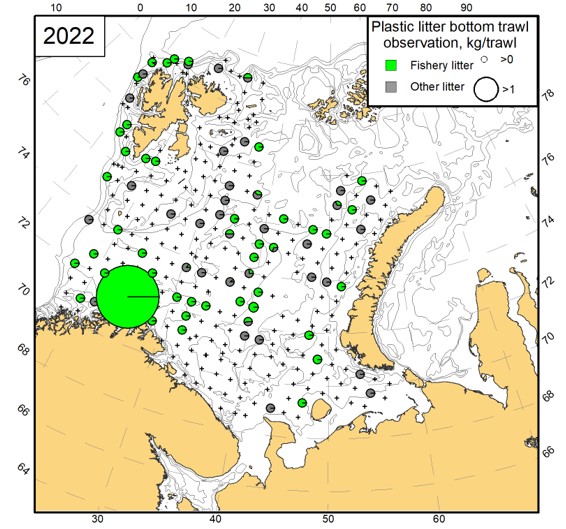
Litter from fishery was a significant part of plastic litter both in the pelagic and bottom trawls (46.2 % and 65.4 % respectively, Fig. 4.2.1.5).
5 - PLANKTON COMMUNITY
5.1 Phytoplankton, chlorophyll a and nutrients
Text by: Sarah Joanne Lerch
Figures by: Sarah Joanne Lerch
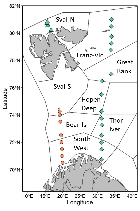
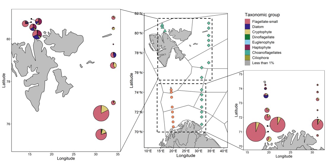
Samples for phytoplankton community composition and abundance were collected from 27 preselected stations along fixed transects in the Barents Sea (Fig. 5.1.1). Samples were collected from Hinlopen and Vardø-N Utvidet during the late summer ecosystem cruise (2022110, 202210), and Fugløya-Bjørnøya during a spring transect cruise (2022207). Phytoplankton samples were collected using two methods, the Algae-net and CTD. Qualitative Algae-net samples were collected using a vertical net tow (10 μm mesh; 0.1 m2 opening; 30-0 m), fixed with 2 ml 20% formalin and stored for future use. Samples for algal cell counts (100 ml) were taken from 10 m CTD collected water and fixed in Neutral Lugol. Microscope counts were performed following the Utermöhl (1958) method on all CTD samples to quantify community composition and abundance at the Flødevigen Plankton Laboratory.
Microscopy counts include heterotrophic and autotrophic groups, these communities will therefore be referred to as microplankton in the summarized results below.
Nutrient and chlorophyll samples were collected from rosette-mounted water-bottles released at various depths at the CTD stations in the Norwegian sector of the Barents Sea. The nutrient samples (20 ml) were preserved with chloroform (200 ml), and thereafter kept at about 4°C until subsequent chemical analysis on shore at IMR. The chlorophyll-samples were collected by filtering 263 ml of seawater through glass-fibre filters, which were then frozen at about -18°C until subsequent extraction of pigments in acetone and thereafter fluorometric analysis in the IMR laboratory on shore. Data on nutrient levels (nitrate, nitrite, silicate and phosphate) are not presented in the cruise-report, but are available at IMR.
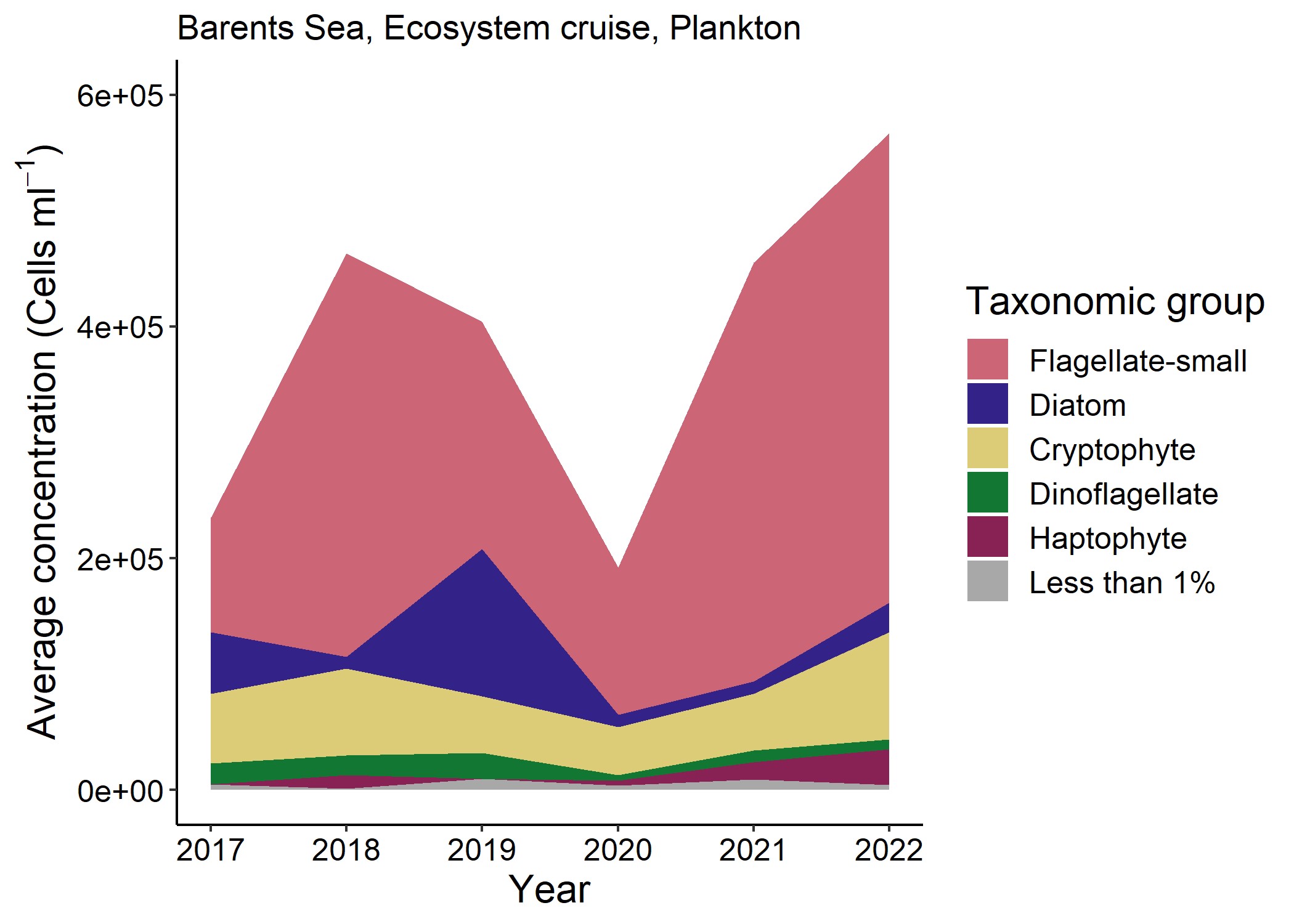
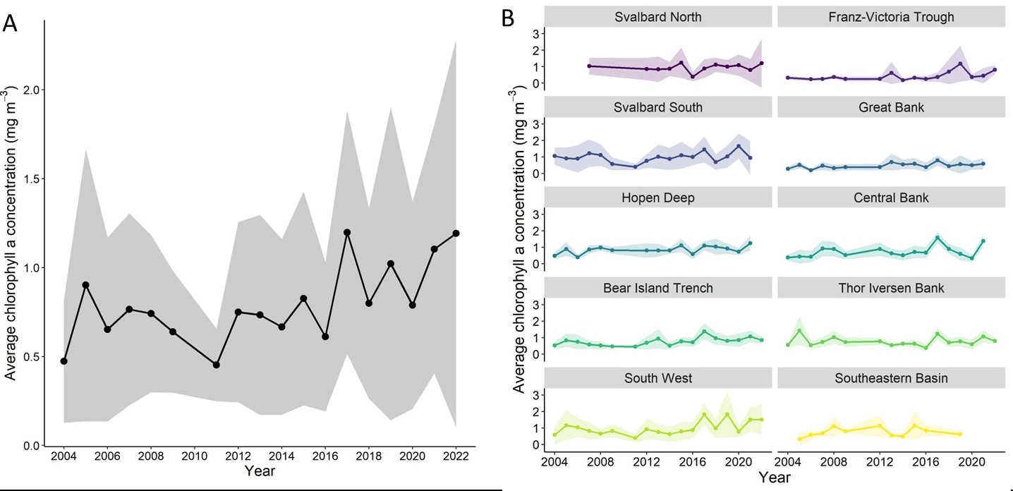
During the ecosystem cruise, the Barents Sea microplankton community at an average station was numerically dominated by small flagellates (71%, 4.1×10⁵ ± 6.4×10⁵ cells ml-1) with smaller contributions from cryptophytes (16%, 9.3×10⁴ ± 7.3×10⁴ cells ml-1), diatoms (5%, 2.6×10⁴ ± 4.7×10⁴ cells ml-1) and haptophytes (5%, 3.1×10⁴ ± 5.2×10⁴ cells ml-1) (Fig. 5.1.2). Small flagellates have consistently comprised at least 42% of the average microplankton community quantified during the ecosystem cruises since 2017. Microplankton community concentration overall has increased since 2020, small flagellates accounted for the majority of this (219% increase) but haptophytes (557%, increase), diatoms (139% increase), and cryptophytes (123% increase) contributed as well. Increasing cell concentrations correspond to increasing average surface chlorophyll concentrations during this period (Fig. 5.1.3). Changes in chlorophyll concentrations since 2020 are also part of a long-term trend of increasing chlorophyll which began in 2010. It should be noted that these patterns are not seen in all ICES sub-regions though, indicating spatial variations in chlorophyll concentrations within the sea.
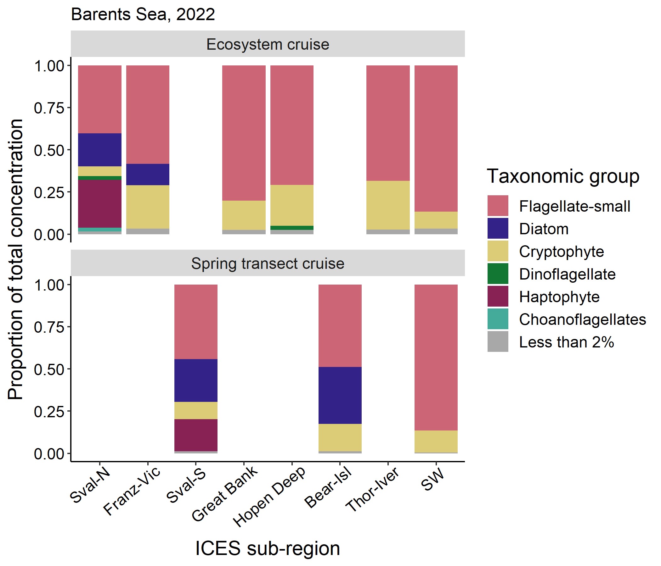
Spatial and temporal variations were also seen within the 2022 microplankton community. During the ecosystem cruise, the taxa which contributed substantially to community composition (≥ 2%) differed in the most Northern ICES-sub regions (Svalbard N and Fanz Victoria Trough) relative to the southern ones (Great Bank, Hopen Deep, Thor Iverson Bank, South West) (Fig. 5.1.4). Diatoms were substantial contributors in both northern sub-regions and haptophytes in Svalbard North only. Latitudinal changes were also seen in the spring community observed on the Fugløya-Bjørnøya transect, with diatoms and haptophytes more abundant in northern ICES sub-regions. Similar communities, dominated by small flagellates and cryptophytes, were observed in the South West sub-region in both spring and late summer.
The average concentration of all microplankton in the late summer (5.65×10⁵ ± 6.73×10⁵ cells ml-1) was approximately one third of that measured in the spring (2.11×10⁶ ± 1.84×10⁶ cells ml-1). During the spring, southern stations were characterized by the highest cell abundance, which was mostly attributed to small flagellates (Fig. 5.1.5). In the late summer, cell concentrations were patchy with both the highest (3.12×10⁶ cells ml-1) and the lowest (6.35×10⁵ cells ml-1) concentrations found along the Vardø-N transect.
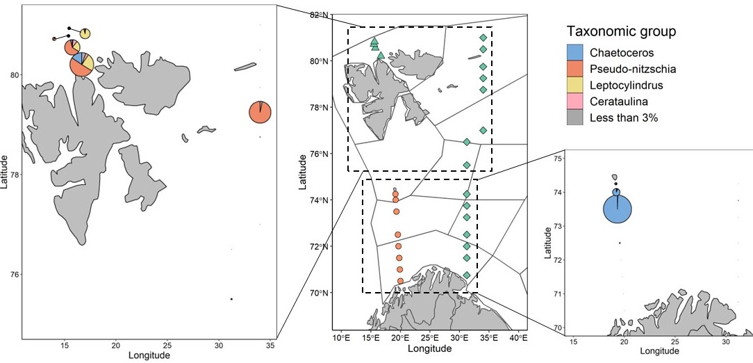
Within the microplankton these data describe only one purely photosynthetic group at a high taxonomic level, diatoms. During the ecosystem cruise, diatom abundance was greatest in the Hinlopen transect (2.0×10⁴-1.44×10⁵ cells ml-1) and most northern Vardø-N station (1.41×10⁴ cells ml-1) (Fig. 5.1.6). These communities were comprised mainly of Pseudo-nitzschia and Leptocylindrus. During the spring, communities were dominated by Chaetoceros and the maximum diatom abundance (8.63×10⁵ cells ml-1) was found in one of the northern Fugløya-Bjørnøya stations.
5.2 Mesozooplankton biomass and geographic distribution
Text by: Espen Bagøien and Irina Prokopchuk
Figure by: E. Bagøien
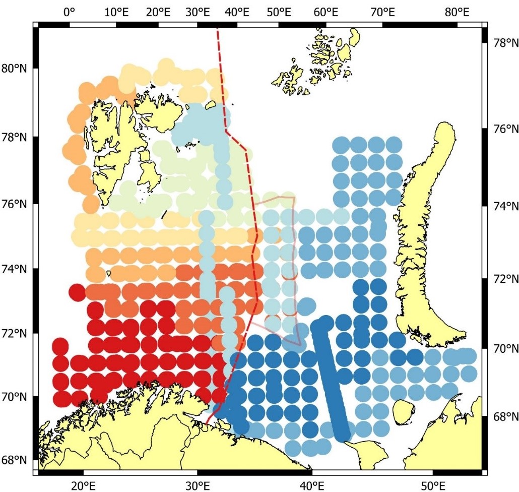
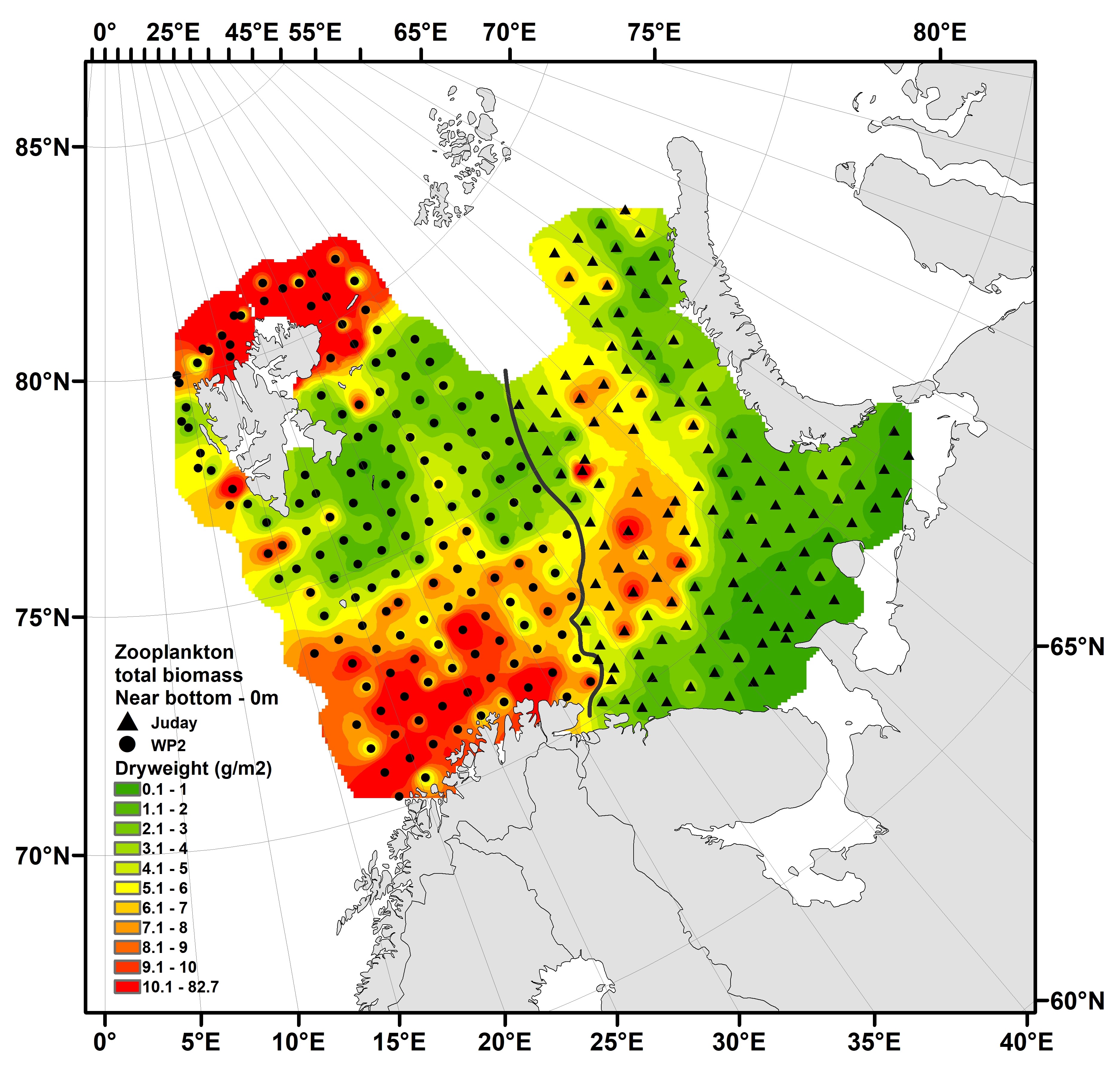
Mesozooplankton sampling stations during the joint Norwegian-Russian Barents Sea ecosystem cruise in 2022 are shown in Figure 5.2.1. In the Norwegian sector the WP2 net (opening area ~ 0.25 m2) was applied, while in the Russian sector the Juday net (opening area ~ 0.11 m2) was used. Both gears were rigged with nets of mesh-size 180 µm and hauled vertically from near the bottom to the surface. The WP2 and Juday nets provide roughly comparable results with respect to mesozooplankton biomass and species composition (Skjoldal et al., 2019). The Norwegian biomass samples are dried before weighing, while the Russian samples are preserved in 4% formalin and their wet-weight determined. Dry-weight is then estimated by dividing the wet-weight with a factor of 5.
The spatial distribution of total mesozooplankton biomass shown in Figure 5.2.1 is based on a total of 291 samples, of which 161 were located in the Norwegian sector and 130 in the Russian sector. Within the Norwegian sector, the average biomass was 6.9 (± 8.9 SD) g dry-weight m-2. The average zooplankton biomass for the samples within the Russian sector was 3.3 (± 3.0 SD) g dry-weight m-2. All stations shown in Figure. 5.2.1 are included in the 2022 biomass averages here presented.
The time of sampling in the Russian sector this year (26. Oct - 1. Dec, 2022) was unusually late in autumn, both compared to the Norwegian sector (17. Aug – 1. Oct, 2022), and the Russian sector in previous years. Hence, the biomass averages for Norwegian and Russian sectors in 2022 are not directly comparable. Likewise, the validity of comparing biomasses within the Russian sector in 2022 with earlier years becomes questionable. Figure 5.2.1 shows horizontally interpolated zooplankton biomasses for the Norwegian and Russian sectors in 2022, but to visualize the issue of differences in sampling time, we have added a line separating the Norwegian and Russian samples. For closely located Norwegian versus Russian stations separated by this line, the difference in sampling-time could vary between ca. 1.5 and 3 months, with the largest differences occurring in the southern area. We note that the lack of synoptic sampling in 2022 may very well be a confounding factor when evaluating zooplankton biomasses in different parts of the Barents Sea.
Comparison of average biomasses across years is also vulnerable to differing area coverages. Challenges in covering the same area over a series of years are inherent in such large-scale monitoring programs, and interannual variation in ice-cover and logistical issues are two of several reasons for this. To improve the regularity of the sampling grid across the survey area in 2022, most stations belonging to the Hinlopen-section north of Svalbard/Spitzbergen and the whole Vardø-North section were omitted when calculating average biomass (excluded from Fig. 5.2.1). Differences in spatial coverage among years, as well as spatial variability in station density within the survey region will impact biomass estimates, and particularly so in an environment characterized by large-scale patterns in biomass distribution. Such challenges fall outside the scope of this cruise-report, but are addressed in other phora, for instance by analysing time-series for spatially consistent sub-areas.
The overall distribution patterns show similarities across years, although some interannual variability is apparent. In 2022 we observed the familiar pattern of comparatively high biomasses in the southwestern region and north of Svalbard/Spitsbergen, as well as the deeper part of the southeastern region. The biomasses were relatively low in the central regions including the bank areas, and very low in the southeastern corner of the Barents Sea and near Novaja Zemlja (Fig. 5.2.1).
Several factors may impact the levels of zooplankton biomass in the Barents Sea;
- Advective supply of zooplankton from the Norwegian Sea
- Local zooplankton production rates – linked to temperature, nutrient conditions and primary production rates
- Predation from carnivorous zooplankters (jellyfish, krill, hyperiids, chaetognaths, etc.)
- Predation from planktivorous fish incl. capelin, young herring, polar cod, juveniles of cod, saithe, haddock, redfish
- Predation from marine mammals and seabirds
References
Skjoldal, H.R., Prokopchuk, I., Bagøien, E., Dalpadado, P., Nesterova, V., Rønning. J., Knutsen, T. 2019. Comparison of Juday and WP2 nets used in joint Norwegian-Russian monitoring of zooplankton in the Barents Sea. Journal of Plankton Research 41:759-769.
5.3 Macrozooplankton
Macrozooplankton will be updated in the IMR-PINRO survey report from the 2023 BESS survey in 2024.
6 - FISH RECRUITEMENT (YOUNG OF THE YEAR)
Figures by: D. Prozorkevich
Area coverage and estimations
In 2022, coverage of the 0-group fish was limited to the western part of the Barents Sea due to technical challenges with Russian vessel (Fig. 6.1). Based on years of full coverage and the average long-term distribution in 2000-2017, we corrected the 2022 abundance indices for lacking coverage. We present species distribution maps for western polygons only.
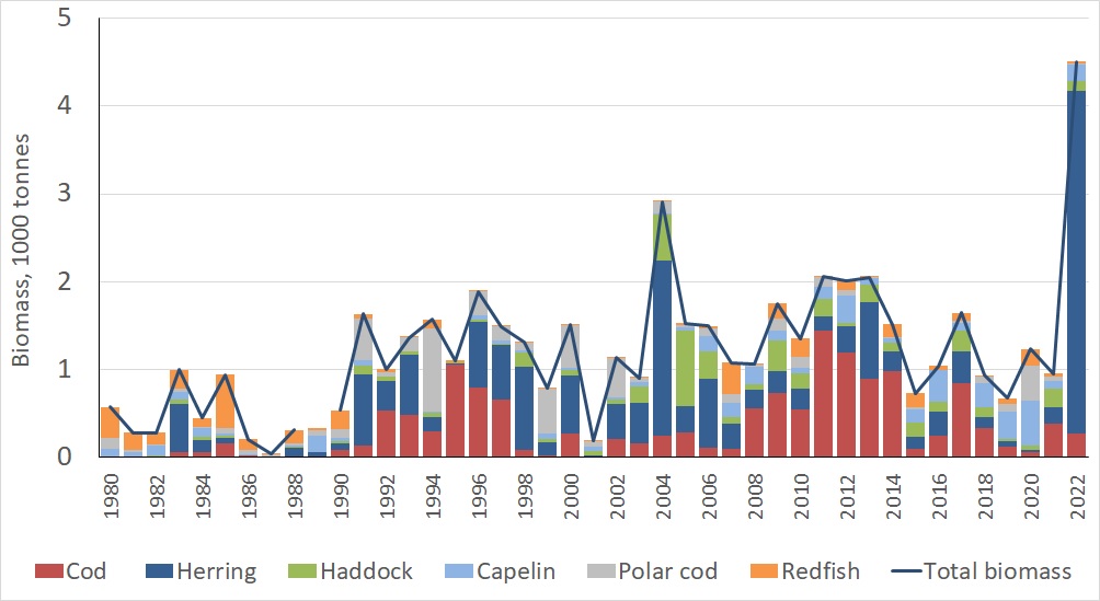
Total biomass
Zero-group fish are important consumers of plankton and are prey for predators (larger fish, sea birds and marine mammals) and, therefore, are important for transfer of energy between trophic levels in the ecosystem. Estimated total biomass of 0-group fish species (cod, haddock, herring, capelin, polar cod, and redfish) varied from a low of 0.165 million tonnes in 2001 to a peak of 4.5 million tonnes in 2022 with a long-term average of 1.2 million tonnes (1993-2022) (Figure 6.2). In 2022, estimated total biomass of 0-group fish species was record high and was 4.5 million tonnes. In 2022, like in 2012-2013, 0-group fish biomasses were dominated by herring. In 2022, like in 2012-2013, 0-group fish biomasses were dominated by herring. In 2022, observed polar cod and capelin biomasses were especially low due to lack of coverage of their distribution areas. The indices are corrected for incomplete area coverage in Figure 6.2.
6.1 Capelin (Mallotus villosus)
The highest average abundance per strata were found in the Svalbard North (435 billion individuals) and Central Bank (17billion individuals) areas.
The 0-group capelin body length varied from 2 to 7.4 cm in 2022, while most of capelin were medium size with body length of 3.5-5.9 cm in 2022, which is similar to length distribution in 2021. Larger individuals (with an average length above 5 cm) were found mainly in northern areas, that indicated most likely that larvae from early spawning drifted further north. The smallest capelin with average length close to 3 cm were found in the southwestern areas (South West).
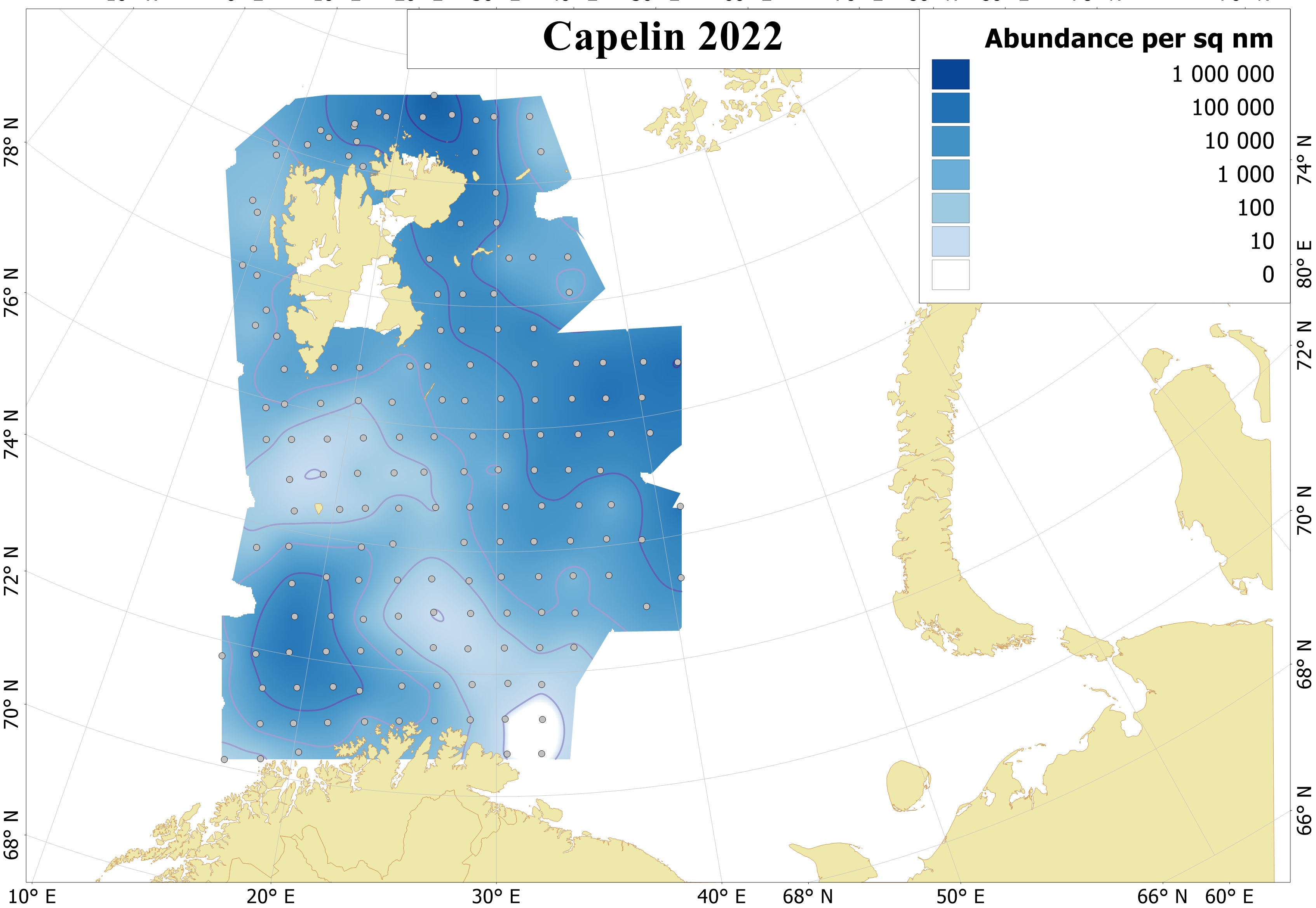
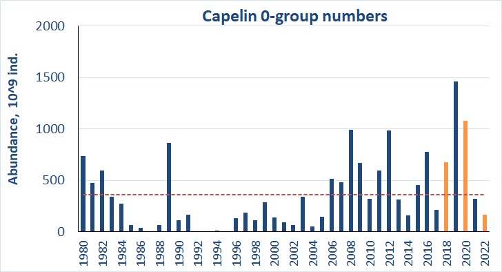
A record strong year class of capelin occurred in 2019, followed by medium (2020), weak (2021) and most likely weak 2022-year classes. Estimated abundance of 0-group capelin varied from 1 billion in 1993 to 1. 5 billion individuals in 2019 with a long-term average of 361.6 billion individuals for the 1980-2022 period (Figure 6.1.2). In 2022, the eastern Barents Sea was not covered, where 0-group capelin were often found, and thus abundance and biomass indices were underestimated. Based on the average long-term distribution in 2000-2017, we corrected the 2022 abundance indices for lacking coverage like in 2018 and 2020. In 2022, the total abundance index for 0-group capelin was well below the long term mean and was 164.6 billion individuals (Fig. 6.1.2). Therefore, the 2022 year-class of capelin seemed to be weak.
However, estimated biomass of 0-group capelin was higher than the long term mean and was 186 thousand tonnes.
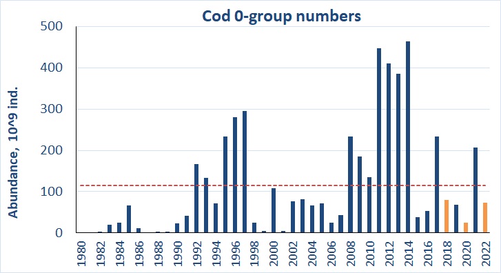
6.2 Cod (Gadus morhua)
The highest average abundance per polygon were found in the northern area (Svalbard North, 18 billion individuals). In 2022, the eastern Barents Sea was not covered, where 0-group cod were usually found, and thus the first abundance indices were underestimated and represents the covered area only.
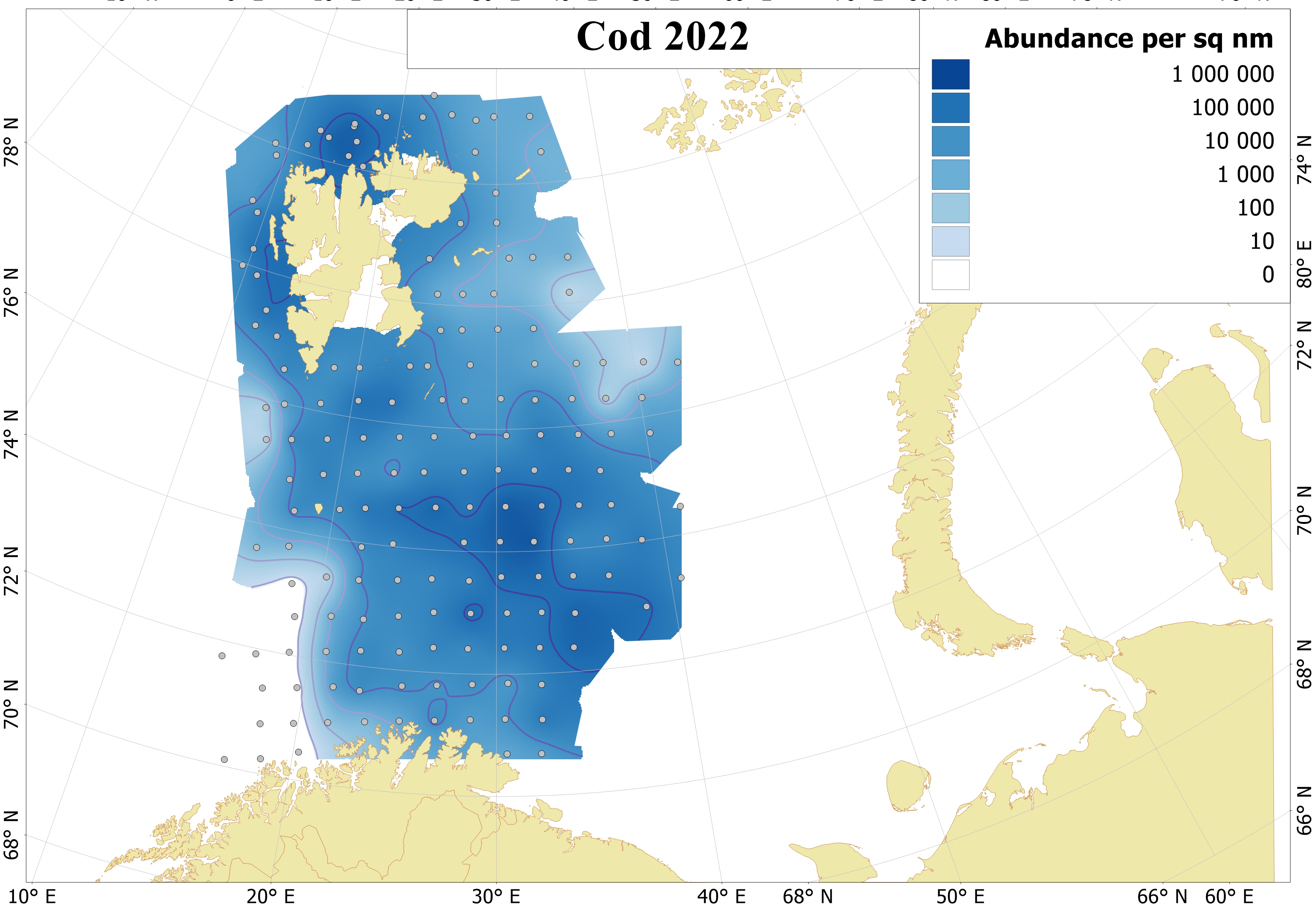
In 2022, 0-group cod were larger than in 2021 and were dominated by fish of 7.0-8.4 cm length. The largest cod (with an average close to 8,5 cm) were observed in polygons of the Southeastern and Great and Central Banks. Some few specimens of small cod below 1.5 cm were found in the Southeastern, Thor Iversen Bank and Svalbard North polygons.
Estimated abundance of 0-group cod varied from 0.276 billion in 1980 to 464.1 billion individuals in 2014 with a long-term average of 114.4 billion individuals for the 1980-2022 period (Figure 3.6.2). In 2022, the total abundance index for 0-group cod was below the long term mean and was 72.8 billion individuals. Cod estimated biomass in 2022 (277 thousand tonnes) was somewhat lower than in 2021 (385 thousand tonnes) and the long term mean for 2003-2022 (339 thousand tonnes). Therefore, the 2022 year-class of cod seemed to be below average.
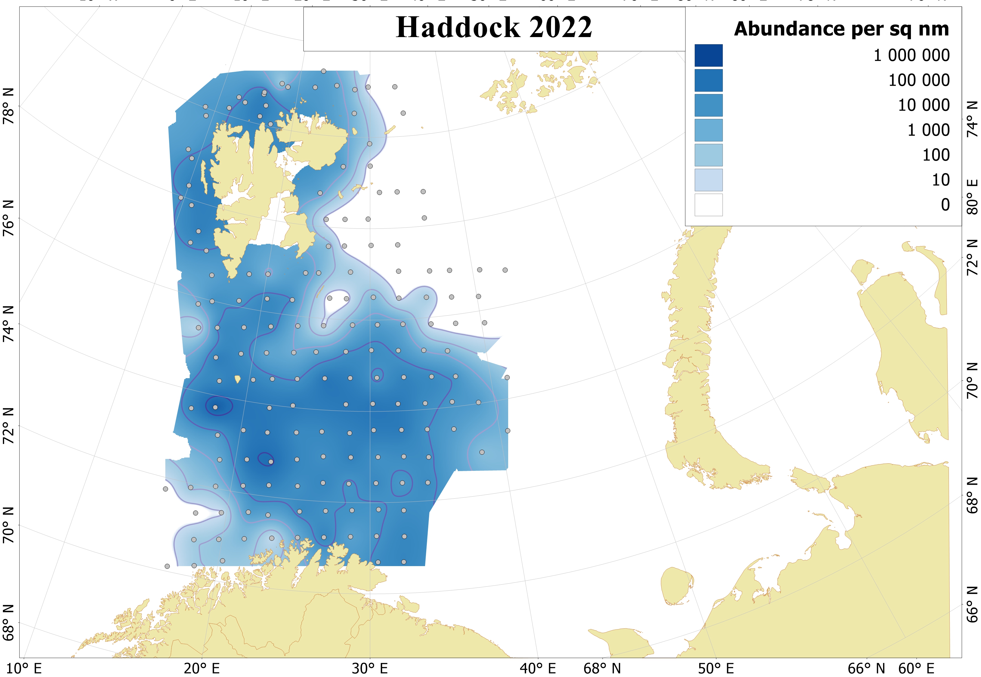
6.3 Haddock (Melanogrammus aeglefinus)
More than half of the 0-group haddock were found in the Bear Island Trench polygon and the abundance there was as high as 11 billion ind. Haddock were also distributed along the western Svalbard/Spitsbergen archipelago (Fig. 6.3.1.).
In 2022, 0-group haddock dominated by fish of 8.0 – 11.4 cm length. The largest haddock (with an average length > 12-13 cm) were observed in the central areas (Great Bank and Southeastern basin), while the smallest haddock were found in the northern areas (with an average length < 6-7 cm).
Estimated abundance of 0-group haddock varied from 0.075 billion in 1982 to 91.6 billion individuals in 2005 with a long-term average of 12.1 billion individuals for the 1980-2022 period (Figure 6.3.2).
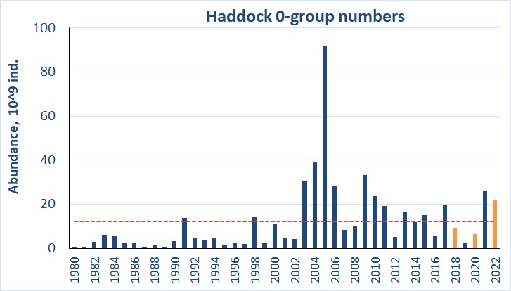
In 2022, the total abundance estimates for 0-group haddock were higher than the long term mean and was 22.1 billion individuals. Haddock estimated biomass in 2022 (124 thousand tonnes) was lower than in 2021 (216 thousand tonnes) and close to the long term mean for 2003-2022 (115 thousand tonnes). Lack of coverage in the eastern Barents Sea will not influence the level of abundance indices so much due to 0-group haddock usually being distributed in the western and central areas. Thus, the 2022-year class may be characterized as strong.
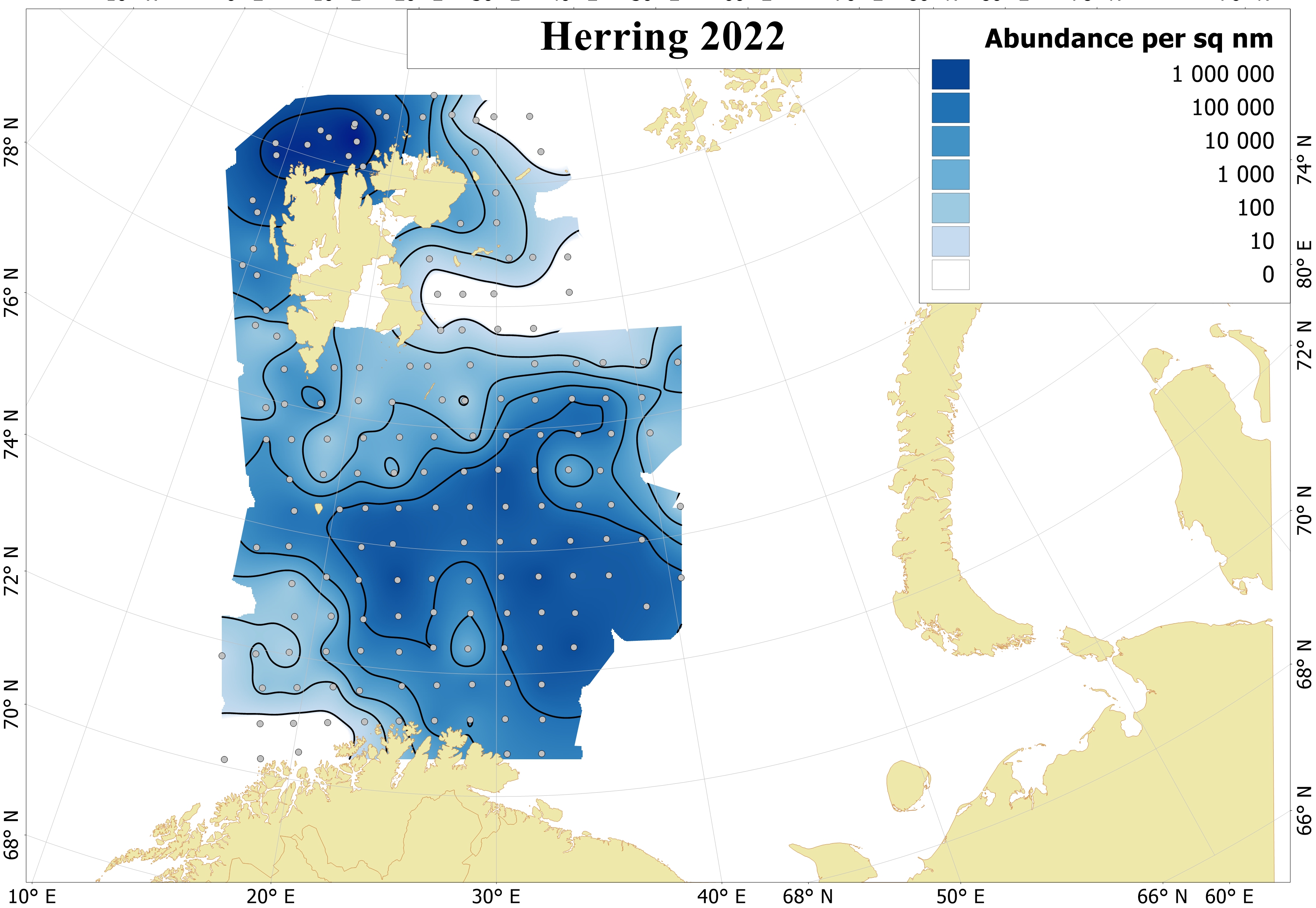
6.4 Herring (Clupea harengus)
0-group herring were widely distributed in the covered area (Fig. 6.4.1). The highest average abundance per polygon were found Svalbard North (1100 billion individuals) and fish of average size (with an average length of 5.6 cm). Relatively high concentrations were also found in the Bear Island Trench, Thor Iversen Bank and Hopen Deep polygons (with an average of 140-160 billions individuals).
The length of the majority of herring (90%) varied between 4 and 7 cm in 2022. Larger individuals were observed in the central areas with an average length of 6.0 cm, while the smallest herring was found in the southeastern areas and north of Svalbard (Spitzbergen).
Estimated abundance of 0-group herring varied from 0.037 billion in 1982 to774 billion individuals in 2004 (Figure 6.4.2). In 2022, the eastern Barents Sea was not fully covered and zero border of herring distribution were not found in the east, and thus abundance and biomass indices estimates are slightly underestimated. Despite this, in 2022, the total abundance index for 0-group herring was almost 10 times higher than to the long term mean and was close to 2000 billion individuals (Figure 6.4.2).
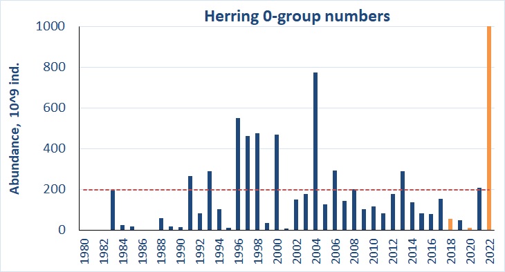
Estimated biomass of 0-group herring was highest since 2004 and much higher than the long-term mean (411 thousand tonnes) and was close to 4 million tonnes. Therefore, the 2022-year class of herring may be characterized as record strong. Unfortunately, half of the 0-group herring abundance was distributed north of Svalbard and therefore their survival during the first winter is highly unknown.
6.5 Polar cod (Boreogadus saida)
Polar cod were found around the Svalbard archipelago in 2022 (Fig. 6.5.1). Coverage of the 0-group polar cod was not complete, especially in the eastern parts of the Barents Sea (Fig. 6.1), and thus the south-eastern component of polar cod could not be presented here.
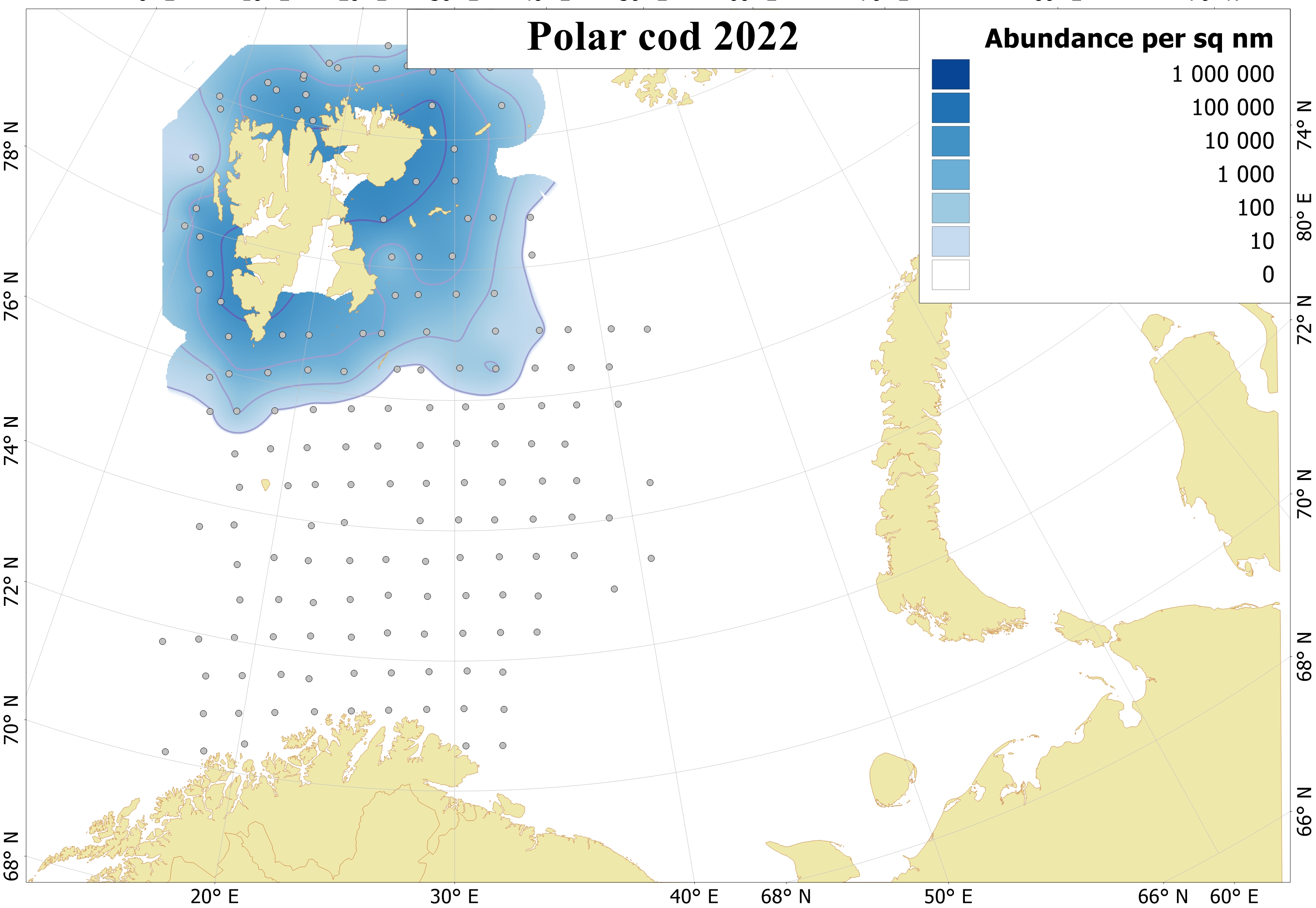
The polar cod length varied between 2.5 and 8.0 cm, while dominated by fish with length of 3.5-5.5 cm. In 2020, the average length was 4.8 cm. Averaged length doesn’t vary between polygons.
Estimated abundance of 0-group polar cod varied from 0.201 billion in 1995 to 2400* billion individuals in 1994 with a long-term average of 307.6 billion individuals for the 1980-2022 period (Figure 3.5.4). In 2018, 2020, 2021 and 2022 the eastern part of the Barents Sea was not fully covered, where 0-group polar cod are often found, and thus abundance and biomass indices were underestimated. The eastern component has dominated in abundance and biomass during 1980, 1990 and early 2000s. In 2022, the total abundance index for 0-group polar cod was extremely low and was 5.4 billion individuals (Figure 6.5.2).
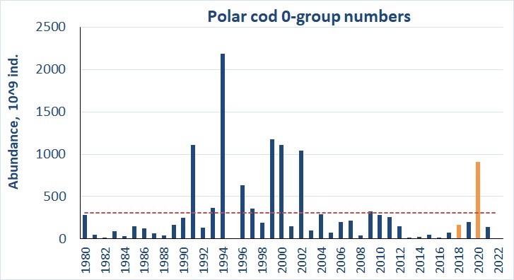
In 2021, estimated biomass of 0-group polar cod was 1/15 of the long term mean (134 thousand tonnes for the period 1993-2022) and was 9 thousand tonnes.
The abundance index of 2022-year class from Svalbard (Spitzbergen) population is very low and may be characterized as weak.
6.6 Saithe (Pollachius virens)
Saithe distribution and abundance varied a lot between years. In 2022, 0-group saithe were found in the central Barents Sea such as in 2021 (Fig. 6.6.1).
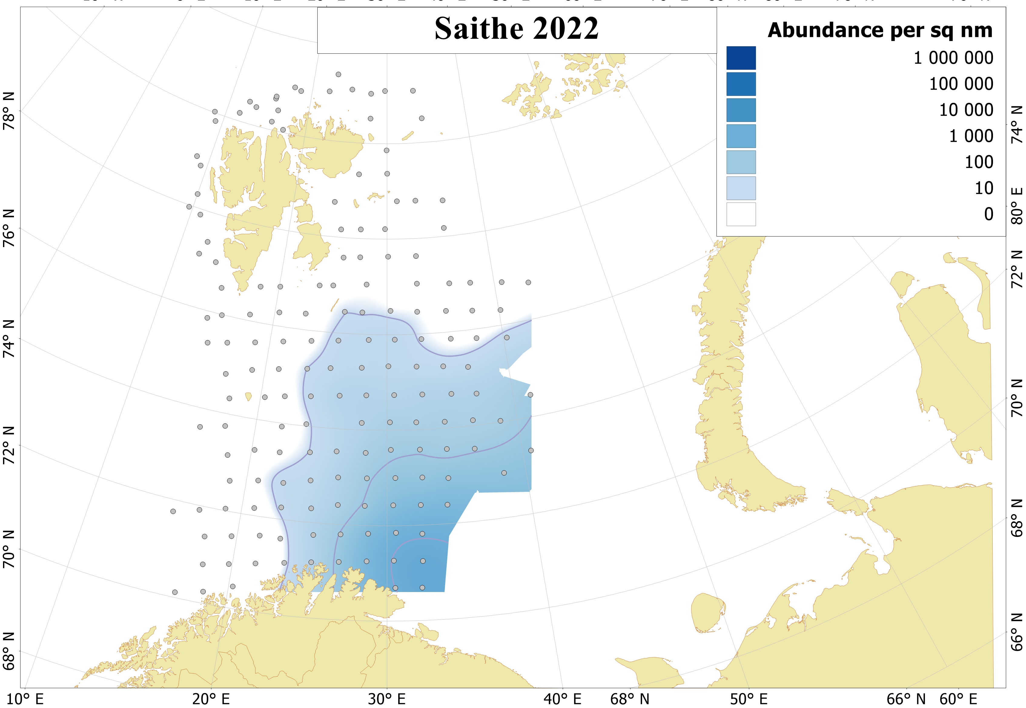
Largest saithe with an average of 11-12 cm were observed in the Bear Island Trench and Thor Iversen Bank polygons, fish with an average of 8.5-9.0 cm were found in the northcentral areas.
In 2022, abundance was higher than long term mean (442 million for the period 1980-2022), i.e. 724 million individuals (Fig. 6.6.2).
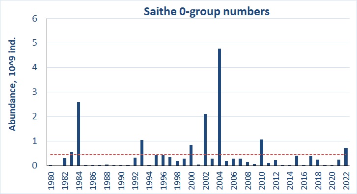
0-group saithe are generally distributed along the Norwegian coast, while some part of the year class are transported to the Barents Sea. Therefore, abundance indices for saithe may not represent year classes strength but give indication of abundance in the Barents Sea.
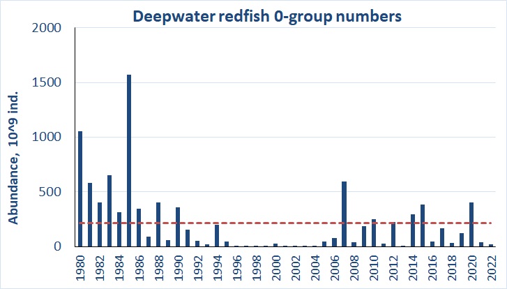
6.7 Redfish (mostly Sebastes mentella)
0-group redfish was distributed from north of Norwegian coast to the northwest/east of Svalbard (Spitsbergen) archipelago in 2022 (Figure 6.7.1). The densest concentrations and the largest fish with an average length of 4.3 cm were found in the Thor Iversen Bank polygon.
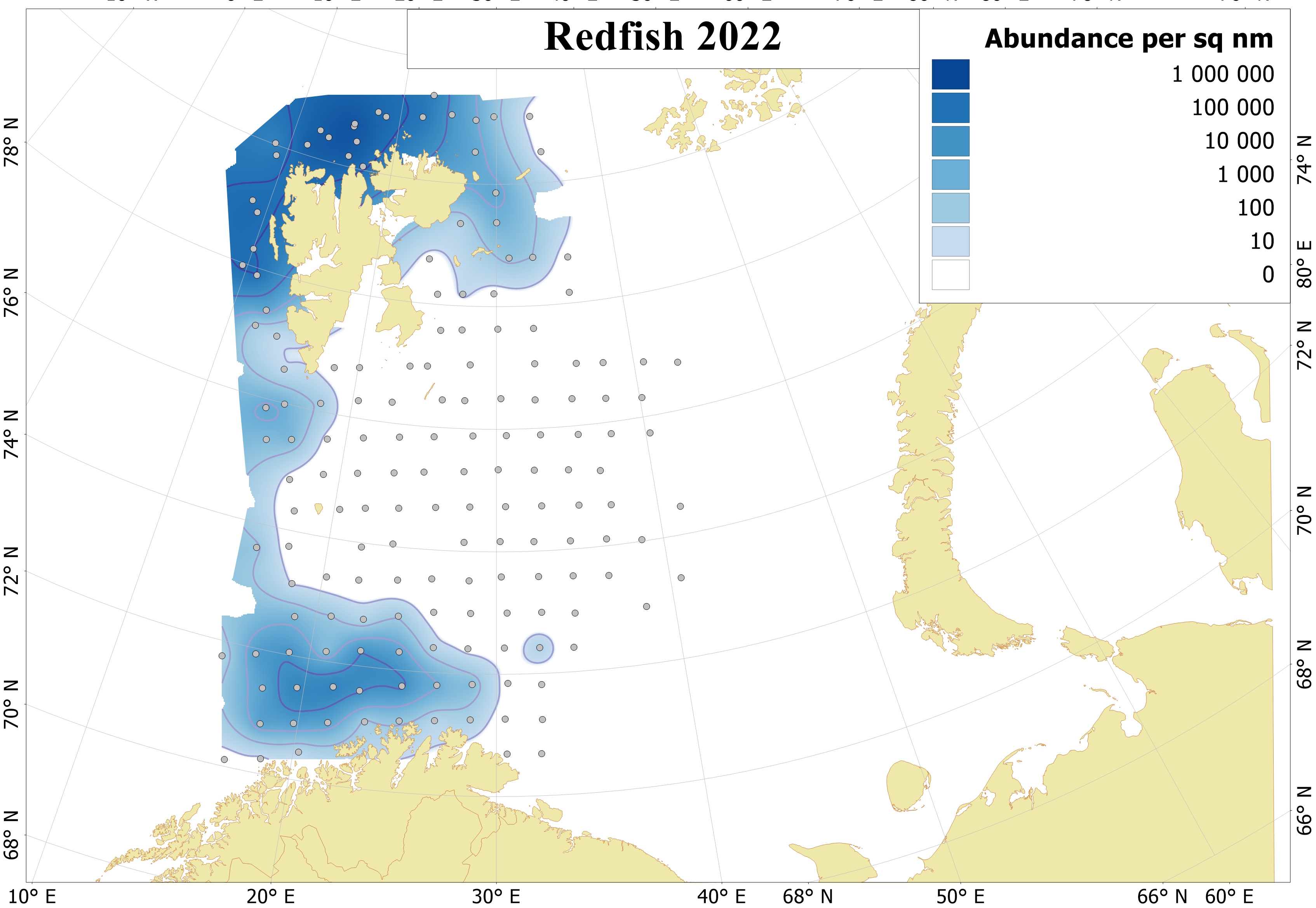
Estimated abundance of 0-group deepwater redfish varied from 23 billion individuals in 2001 to 1600 billion individuals in 1985, and long term average abundance was 217 billion individuals for the 1980-2022 period (Figure 6.7.2). In 2022, the total abundance index for 0-group deepwater redfish was very low and was 9.1 billion individuals, which is much lower than the long-term mean. The total biomass was close to 19 thousand tonnes. Thus the 2022-year class may be characterized as weak.
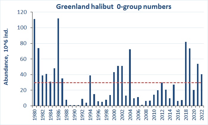
6.8 Greenland halibut (Reinhardtius hippoglossoides)
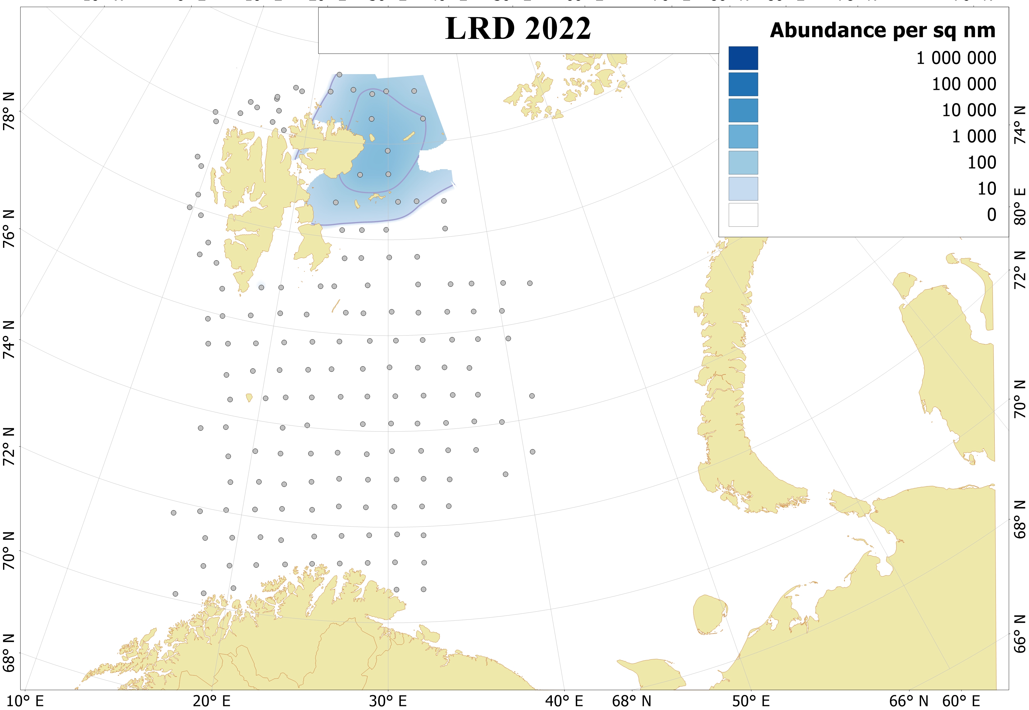
0-group Greenland halibut were found distributed around the Svalbard (Spitzbergen) in 2022 similar to the distribution in 2018-2021 (Figure 6.8.1).
0-group Greenland halibut length varied from 2.5 to 9.5 cm. Larger fish were found in the Fr.Victoria Trough polygon, and fish length were with an average of 7.3 cm, while smaller fish were found in the Svalbard South and Svalbard North polygons with an average of 6.6 - 6.7 cm.
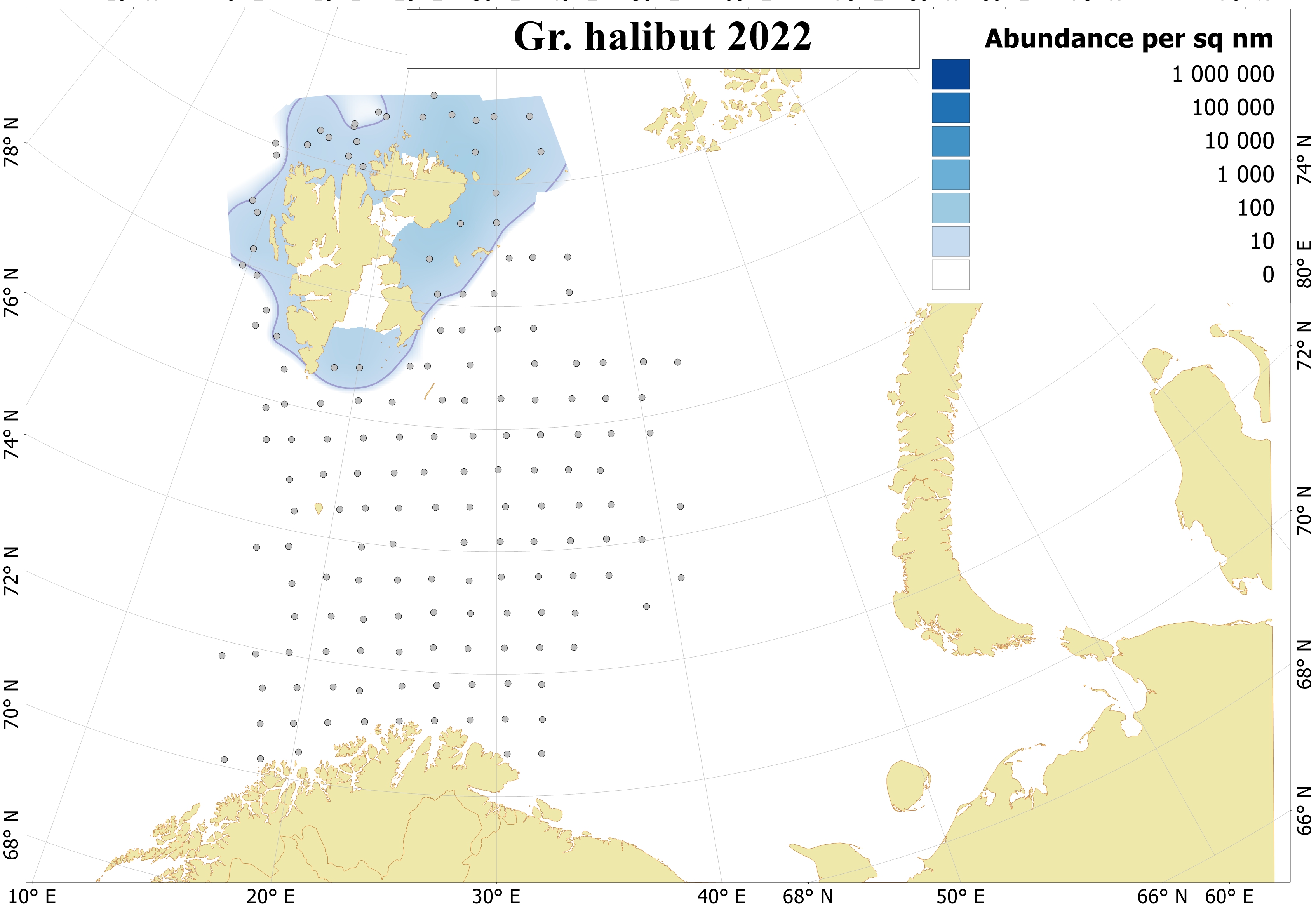
In 2022, the total abundance index for 0-group fish were 40.5 *106 individuals, that was higher than the long term mean of 30 million individuals. Estimated biomass was also higher than the long term mean (of 82 tonnes) and was 73 tonnes.
6.9 Long rough dab (Hippoglossoides platessoides)
In 2022, 0-group long rough dab were mainly distributed in the north of Svalbard (Spitsbergen) (Figure 6.9.1). In 2022, the eastern Barents Sea was not covered, where long rough dab is usually distributed.
The 0-group long rough dab length varied from 0.5 to 6.0 cm with an average of 3.9 cm.
In 2022, the total abundance index for 0-group fish were 69.3 million individuals that was lowest since 2014. Estimated biomass was also lower than long term mean of 287 tonnes and was 48 tonnes.
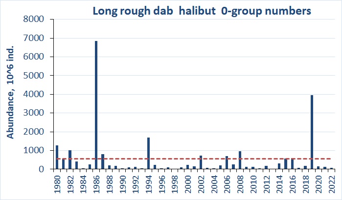
Thus the 2022-year class of long rough dab is difficult to characterize because lack of coverage in traditional area.
7 - COMMERCIAL PELAGIC FISH
Figures by S. Karlson, G. Skaret
In 2022, the Russian survey sector was surveyed with a significant delay (see chapter 2). Thus, initially the calculations of numbers and biomass were made for the Norwegian part only.
7.1 Capelin (Mallotus villosus)
Only the Norwegian side of the Barents Sea was covered synoptically, the eastern part of the feeding area for capelin was covered late (see Figure 7.1.1.1). It is highly variable between years how much capelin is present in the eastern part of the distribution area (see: Advice on fishing opportunities for Barents Sea capelin in 2023 | Havforskningsinstituttet). Assesment in October-November cannot be combined with assesment in August-September, since there are no reliable data on capelin migration within 2 months. Therefore, the estimates given in the table 7.1.2.1b can only be used as additional information.
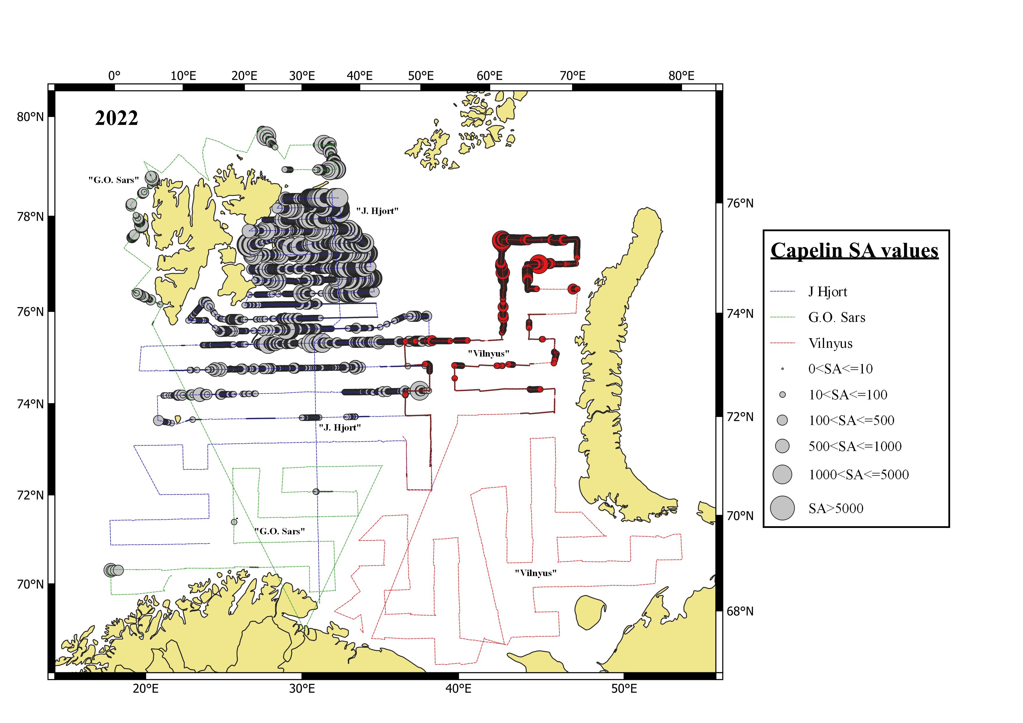
7.1.1 Geographical distribution
The Norwegian (western) side of the Barents Sea was covered during BESS in August-September 2022, and the geographical distribution of capelin recorded acoustically is shown in Figure 7.1.1.1 (marked in gray colour). The capelin was distributed further north than in recent years. Significant recordings of capelin were made north of Kvitøya already in early September by ‘GO Sars’. A similar northerly distribution has not been observed since 2013. The Russian (eastern) part was covered in October-November. Capelin was distributed far to the northeast up to 78°N and 60°E (see Figure 7.1.1.1, marked in red). The main densities were found at the border of the surveyed area, which shows that the capelin distribution was even further north and east.
7.1.2 Abundance by size and age
A detailed summary of the acoustic stock estimate is given in Table 7.1.2.1a, and the time series of abundance estimates is summarized in Table 7.1.2.2. A comparison between the estimates in 2022 and 2021 is given in the table 7.1.2.3 with the 2021 estimate shown on a shaded background.
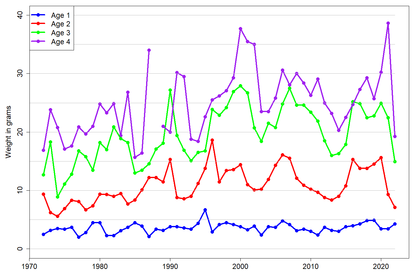
The total stock in the covered area was estimated to about 2.17 million tons, which is below the long-term average level (2.8 million tons). About 38 % (0.82 million tons) of the 2022 stock had length above 14 cm and was therefore considered to be maturing. The 2-year-olds and 3-year-olds (2020 and 2019 year-classes) dominated in the capelin stock in terms of both abundance and biomass. Late estimation in October-November in the northeastern part showed a SSB in this area of about 244 thousand tons. There was a significant dominance of age 3+ (70%). Average weight at age (based on the western survey area) was the lowest since the 1970s for the 2-year-olds and the lowest since the mid-eighties for 3-year-olds (figure 7.1.2.1).
The work concerning assessment and quota advice for capelin is dealt with in a separate report published here: Advice on fishing opportunities for Barents Sea capelin in 2023 | Havforskningsinstituttet.
|
Length (cm) |
Age/year class |
Sum (109) |
Biomass (103 t) |
Mean weight (g) |
||||
|
1 |
2 |
3 |
4 |
5 |
||||
|
2021 |
2020 |
2019 |
2018 |
2017 |
||||
|
7.0-7.5 |
0.275 |
|
|
|
|
0.275 |
0.347 |
1.26 |
|
7.5-8.0 |
0.448 |
|
|
|
|
0.448 |
0.982 |
2.19 |
|
8.0-8.5 |
1.851 |
|
|
|
|
1.851 |
4.324 |
2.34 |
|
8.5-9.0 |
3.240 |
|
|
|
|
3.240 |
9.512 |
2.94 |
|
9.0-9.5 |
11.849 |
0.367 |
|
|
|
12.216 |
41.061 |
3.36 |
|
9.5-10.0 |
16.198 |
0.643 |
|
|
|
16.841 |
64.576 |
3.83 |
|
10.0-10.5 |
18.004 |
3.259 |
0.234 |
|
|
21.498 |
92.273 |
4.29 |
|
10.5-11.0 |
15.478 |
22.005 |
0.997 |
|
|
38.481 |
191.589 |
4.98 |
|
11.0-11.5 |
4.450 |
28.864 |
1.244 |
|
|
34.558 |
193.871 |
5.61 |
|
11.5-12.0 |
2.061 |
28.342 |
2.699 |
|
|
33.102 |
211.645 |
6.39 |
|
12.0-12.5 |
1.194 |
20.241 |
4.766 |
|
|
26.201 |
190.108 |
7.26 |
|
12.5-13.0 |
0.270 |
11.627 |
3.362 |
0.016 |
|
15.275 |
128.200 |
8.39 |
|
13.0-13.5 |
0.141 |
8.034 |
4.325 |
0.081 |
|
12.581 |
122.333 |
9.72 |
|
13.5-14.0 |
|
4.171 |
5.232 |
0.068 |
|
9.470 |
105.374 |
11.13 |
|
14.0-14.5 |
|
2.936 |
5.955 |
0.040 |
|
8.932 |
114.229 |
12.79 |
|
14.5-15.0 |
|
1.788 |
5.060 |
0.046 |
|
6.894 |
101.479 |
14.72 |
|
15.0-15.5 |
|
1.294 |
5.544 |
0.262 |
|
7.100 |
119.397 |
16.82 |
|
15.5-16.0 |
|
0.832 |
5.340 |
0.184 |
|
6.356 |
122.091 |
19.21 |
|
16.0-16.5 |
|
0.933 |
5.625 |
0.447 |
|
7.006 |
148.635 |
21.22 |
|
16.5-17.0 |
|
0.290 |
3.518 |
0.005 |
|
3.814 |
91.257 |
23.93 |
|
17.0-17.5 |
|
0.079 |
1.988 |
0.077 |
|
2.143 |
59.219 |
27.63 |
|
17.5-18.0 |
|
0.078 |
1.019 |
0.025 |
0.008 |
1.129 |
34.809 |
30.82 |
|
18.0-18.5 |
|
0.004 |
0.679 |
|
|
0.683 |
22.707 |
33.24 |
|
18.5-19.0 |
|
|
0.103 |
|
|
0.103 |
3.620 |
35.20 |
|
19.0-19.5 |
|
|
0.001 |
|
|
0.001 |
0.033 |
39.00 |
|
TSN (109) |
75.460 |
135.787 |
57.692 |
1.250 |
0.008 |
270.197 |
|
|
|
TSB (103 t) |
324.674 |
964.078 |
860.680 |
24.052 |
0.188 |
|
2173.671 |
|
|
Mean length (cm) |
9.85 |
11.69 |
14.22 |
15.32 |
17.50 |
11.98 |
|
|
|
Mean weight (g) |
4.30 |
7.10 |
14.92 |
19.25 |
24.00 |
|
|
8.04 |
|
SSN (109) |
0 |
8.234 |
34.833 |
1.085 |
0.008 |
44.160 |
|
|
|
SSB (103 t) |
0 |
133.063 |
662.616 |
21.613 |
0.241 |
|
817.476 |
|
Target strength estimation based on formula: TS= 19.1 log (L) – 74.0
|
Length (cm) |
Age/year class |
Sum (109) |
Biomass (103 t) |
Mean weight (g) |
||||
|
1 |
2 |
3 |
4 |
|
||||
|
2021 |
2020 |
2019 |
2018 |
|
||||
|
9.0-9.5 |
0.505 |
|
|
|
|
0.505 |
1.045 |
2.07 |
|
9.5-10.0 |
0.454 |
|
|
|
|
0.454 |
1.181 |
2.6 |
|
10.0-10.5 |
0.293 |
|
|
|
|
0.293 |
0.966 |
3.3 |
|
10.5-11.0 |
0.038 |
|
|
|
|
0.038 |
0.158 |
4.1 |
|
11.0-11.5 |
0.050 |
|
|
|
|
0.050 |
0.225 |
4.51 |
|
11.5-12.0 |
0.422 |
|
|
|
|
0.422 |
2.261 |
5.36 |
|
12.0-12.5 |
|
0.469 |
|
|
|
0.469 |
2.920 |
6.22 |
|
12.5-13.0 |
|
1.460 |
0.422 |
|
|
1.882 |
13.325 |
7.08 |
|
13.0-13.5 |
|
1.417 |
0.000 |
|
|
1.417 |
11.349 |
8.01 |
|
13.5-14.0 |
|
1.388 |
0.657 |
|
|
2.045 |
19.198 |
9.39 |
|
14.0-14.5 |
|
0.704 |
1.292 |
|
|
1.996 |
23.375 |
11.71 |
|
14.5-15.0 |
|
0.485 |
1.150 |
|
|
1.635 |
20.173 |
12.34 |
|
15.0-15.5 |
|
0.560 |
1.396 |
|
|
1.956 |
29.239 |
14.95 |
|
15.5-16.0 |
|
0.211 |
1.341 |
|
|
1.552 |
27.165 |
17.5 |
|
16.0-16.5 |
|
|
1.333 |
0.199 |
|
1.532 |
30.653 |
20.01 |
|
16.5-17.0 |
|
|
0.777 |
|
|
0.777 |
18.074 |
23.27 |
|
17.0-17.5 |
|
|
0.572 |
|
|
0.572 |
14.584 |
25.49 |
|
17.5-18.0 |
|
|
0.447 |
0.081 |
|
0.528 |
15.890 |
30.09 |
|
18.0-18.5 |
|
|
0.359 |
|
|
0.359 |
11.054 |
30.82 |
|
18.5-19.0 |
|
|
0.022 |
|
|
0.022 |
0.764 |
34.32 |
|
19.0-19.5 |
|
|
0.014 |
|
|
0.014 |
0.509 |
37.6 |
|
19.5-20.0 |
|
|
0.001 |
|
|
0.001 |
0.061 |
42.19 |
|
TSN (109) |
1.762 |
6.695 |
9.782 |
0.280 |
|
18.518 |
|
|
|
TSB (103 t) |
5.836 |
63.938 |
167.984 |
6.411 |
|
|
244.168 |
|
|
Mean length (cm) |
10.23 |
13.63 |
15.53 |
16.68 |
|
14.36 |
|
|
|
Mean weight (g) |
3.31 |
9.55 |
17.17 |
22.91 |
|
|
|
13.19 |
|
SSN (109) |
0 |
1.960 |
8.703 |
0.280 |
|
10.944 |
|
|
|
SSB (103 t) |
0 |
26.300 |
158.830 |
6.411 |
|
191.540 |
|
|
Target strength estimation based on formula: TS= 19.1 log (L) – 74.0
|
Year |
Age |
Sum |
|||||||||
|
1 |
2 |
3 |
4 |
5 |
|||||||
|
B |
AW |
B |
AW |
B |
AW |
B |
AW |
B |
AW |
B |
|
|
1973 |
1.69 |
3.2 |
2.32 |
6.2 |
0.73 |
18.3 |
0.41 |
23.8 |
0.0 1 |
30.1 |
5.14 |
|
1974 |
1.06 |
3.5 |
3.06 |
5.6 |
1.53 |
8.9 |
0.07 |
20.8 |
+ |
25.0 |
5.73 |
|
1975 |
0.65 |
3.4 |
2.39 |
6.9 |
3.27 |
11.1 |
1.48 |
17.1 |
0.01 |
31.0 |
7.81 |
|
1976 |
0.78 |
3.7 |
1.92 |
8.3 |
2.09 |
12.8 |
1.35 |
17.6 |
0.27 |
21.7 |
6.42 |
|
1977 |
0.72 |
2.0 |
1.41 |
8.1 |
1.66 |
16.8 |
0.84 |
20.9 |
0.17 |
22.9 |
4.80 |
|
1978 |
0.24 |
2.8 |
2.62 |
6.7 |
1.20 |
15.8 |
0.17 |
19.7 |
0.02 |
25.0 |
4.25 |
|
1979 |
0.05 |
4.5 |
2.47 |
7.4 |
1.53 |
13.5 |
0.10 |
21.0 |
+ |
27.0 |
4.16 |
|
1980 |
1.21 |
4.5 |
1.85 |
9.4 |
2.83 |
18.2 |
0.82 |
24.8 |
0.01 |
19.7 |
6.71 |
|
1981 |
0.92 |
2.3 |
1.83 |
9.3 |
0.82 |
17.0 |
0.32 |
23.3 |
0.01 |
28.7 |
3.90 |
|
1982 |
1.22 |
2.3 |
1.33 |
9.0 |
1.18 |
20.9 |
0.05 |
24.9 |
|
|
3.78 |
|
1983 |
1.61 |
3.1 |
1.90 |
9.5 |
0.72 |
18.9 |
0.01 |
19.4 |
|
|
4.23 |
|
1984 |
0.57 |
3.7 |
1.43 |
7.7 |
0.88 |
18.2 |
0.08 |
26.8 |
|
|
2.96 |
|
1985 |
0.17 |
4.5 |
0.40 |
8.4 |
0.27 |
13.0 |
0.01 |
15.7 |
|
|
0.86 |
|
1986 |
0.02 |
3.9 |
0.05 |
10.1 |
0.05 |
13.5 |
+ |
16.4 |
|
|
0.12 |
|
1987 |
0.08 |
2.1 |
0.02 |
12.2 |
+ |
14.6 |
+ |
34.0 |
|
|
0.10 |
|
1988 |
0.07 |
3.4 |
0.35 |
12.2 |
+ |
17.1 |
|
|
|
|
0.43 |
|
1989 |
0.61 |
3.2 |
0.20 |
11.5 |
0.05 |
18.1 |
+ |
21.0 |
|
|
0.86 |
|
1990 |
2.66 |
3.8 |
2.72 |
15.3 |
0.44 |
27.2 |
+ |
20.0 |
|
|
5.83 |
|
1991 |
1.52 |
3.8 |
5.10 |
8.8 |
0.64 |
19.4 |
0.04 |
30.2 |
|
|
7.29 |
|
1992 |
1.25 |
3.6 |
1.69 |
8.6 |
2.17 |
16.9 |
0.04 |
29.5 |
|
|
5.15 |
|
1993 |
0.01 |
3.4 |
0.48 |
9.0 |
0.26 |
15.1 |
0.05 |
18.8 |
|
|
0.80 |
|
1994 |
0.09 |
4.4 |
0.04 |
11.2 |
0.07 |
16.5 |
+ |
18.4 |
|
|
0.20 |
|
1995 |
0.05 |
6.7 |
0.11 |
13.8 |
0.03 |
16.8 |
0.01 |
22.6 |
|
|
0.19 |
|
1996 |
0.24 |
2.9 |
0.22 |
18.6 |
0.05 |
23.9 |
+ |
25.5 |
|
|
0.50 |
|
1997 |
0.42 |
4.2 |
0.45 |
11.5 |
0.04 |
22.9 |
+ |
26.2 |
|
|
0.91 |
|
1998 |
0.81 |
4.5 |
0.98 |
13.4 |
0.25 |
24.2 |
0.02 |
27.1 |
+ |
29.4 |
2.06 |
|
1999 |
0.65 |
4.2 |
1.38 |
13.6 |
0.71 |
26.9 |
0.03 |
29.3 |
|
|
2.77 |
|
2000 |
1.70 |
3.8 |
1.59 |
14.4 |
0.95 |
27.9 |
0.08 |
37.7 |
|
|
4.27 |
|
2001 |
0.37 |
3.3 |
2.40 |
11.0 |
0.81 |
26.7 |
0.04 |
35.5 |
+ |
41.4 |
3.63 |
|
2002 |
0.23 |
3.9 |
0.92 |
10.1 |
1.04 |
20.7 |
0.02 |
35.0 |
|
|
2.21 |
|
2003 |
0.20 |
2.4 |
0.10 |
10.2 |
0.20 |
18.4 |
0.03 |
23.5 |
|
|
0.53 |
|
2004 |
0.20 |
3.8 |
0.29 |
11.9 |
0.12 |
21.5 |
0.02 |
23.5 |
+ |
26.3 |
0.63 |
|
2005 |
0.10 |
3.7 |
0.19 |
14.3 |
0.04 |
20.8 |
+ |
25.8 |
|
|
0.32 |
|
2006 |
0.29 |
4.8 |
0.35 |
16.1 |
0.14 |
24.8 |
0.01 |
30.6 |
+ |
36.5 |
0.79 |
|
2007 |
0.93 |
4.2 |
0.85 |
15.5 |
0.10 |
27.5 |
+ |
28.1 |
|
|
2.12 |
|
2008 |
0.97 |
3.1 |
2.80 |
12.1 |
0.61 |
24.6 |
0.05 |
30.0 |
|
|
4.43 |
|
2009 |
0.42 |
3.4 |
1.82 |
10.9 |
1.51 |
24.6 |
0.01 |
28.4 |
|
|
3.77 |
|
2010 |
0.74 |
3.0 |
1.30 |
10.2 |
1.43 |
23.4 |
0.02 |
26.3 |
|
|
3.50 |
|
2011 |
0.50 |
2.4 |
1.76 |
9.7 |
1.21 |
21.9 |
0.23 |
29.1 |
|
|
3.71 |
|
2012 |
0.54 |
3.7 |
1.37 |
8.8 |
1.62 |
18.5 |
0.06 |
25.0 |
|
|
3.59 |
|
2013 |
1.04 |
3.2 |
1.81 |
8.4 |
0.94 |
16.0 |
0.16 |
23.2 |
+ |
29.1 |
3.96 |
|
2014 |
0.32 |
3.0 |
0.95 |
9.0 |
0.64 |
16.3 |
0.04 |
20.3 |
|
|
1.95 |
|
2015 |
0.14 |
3.8 |
0.40 |
10.8 |
0.20 |
17.9 |
0.09 |
22.5 |
+ |
28.1 |
0.84 |
|
2016 |
0.12 |
3.9 |
0.12 |
15.3 |
0.08 |
25.2 |
+ |
24.7 |
|
|
0.33 |
|
2017 |
0.37 |
4.3 |
1.70 |
13.8 |
0.42 |
24.9 |
0.01 |
27.3 |
|
|
2.51 |
|
2018 |
0.29 |
4.9 |
0.80 |
13.8 |
0.48 |
22.4 |
0.01 |
29.3 |
|
|
1.60 |
|
2019 |
0.09 |
4.9 |
0.13 |
14.5 |
0.16 |
22.8 |
0.03 |
25.7 |
|
|
0.41 |
|
2020 |
1.27 |
3.5 |
0.49 |
15.6 |
0.10 |
24.9 |
0.03 |
30.2 |
+ |
22.6 |
1.88 |
|
2021 |
0.76 |
3.4 |
3.08 |
9.3 |
0.16 |
22.5 |
+ |
38.7 |
|
|
4.00 |
|
2022 |
0.32 |
4.3 |
0.96 |
7.1 |
0.86 |
14.9 |
0.02 |
19.2 |
+ |
24.0 |
2.17 |
|
Average |
0.63 |
3.6 |
1.30 |
10.9 |
0.78 |
19.7 |
0.17 |
25.2 |
0.07 |
27.6 |
2.82 |
Note:«+» <0.01*109 tons
Table 7.1.2.3. Summary of acoustic stock size estimates for capelin in 2021-2022.
A comparison between the estimates this year and last year (shaded background).
|
Year class |
Age |
Numbers (106) |
Mean weight (g) |
Biomass (103 t) |
||||
|
2021 |
2020 |
1 |
75.5 |
220.8 |
4.30 |
3.43 |
324.7 |
757.7 |
|
2020 |
2019 |
2 |
135.8 |
329.9 |
7.10 |
9.34 |
964.1 |
3081.5 |
|
2019 |
2018 |
3 |
57.7 |
7.0 |
14.92 |
22.47 |
860.7 |
157.2 |
|
2018 |
2017 |
4 |
1.2 |
0.1 |
19.25 |
38.66 |
24.1 |
1.2 |
|
Total stock in: |
|
|
|
|
|
|
|
|
|
2022 |
2021 |
1-4 |
270.2 |
557.9 |
8.04 |
7.17 |
2173.7 |
3997.8 |
7.2 Polar cod (Boreogadus saida)
7.2.1 Geographical distribution
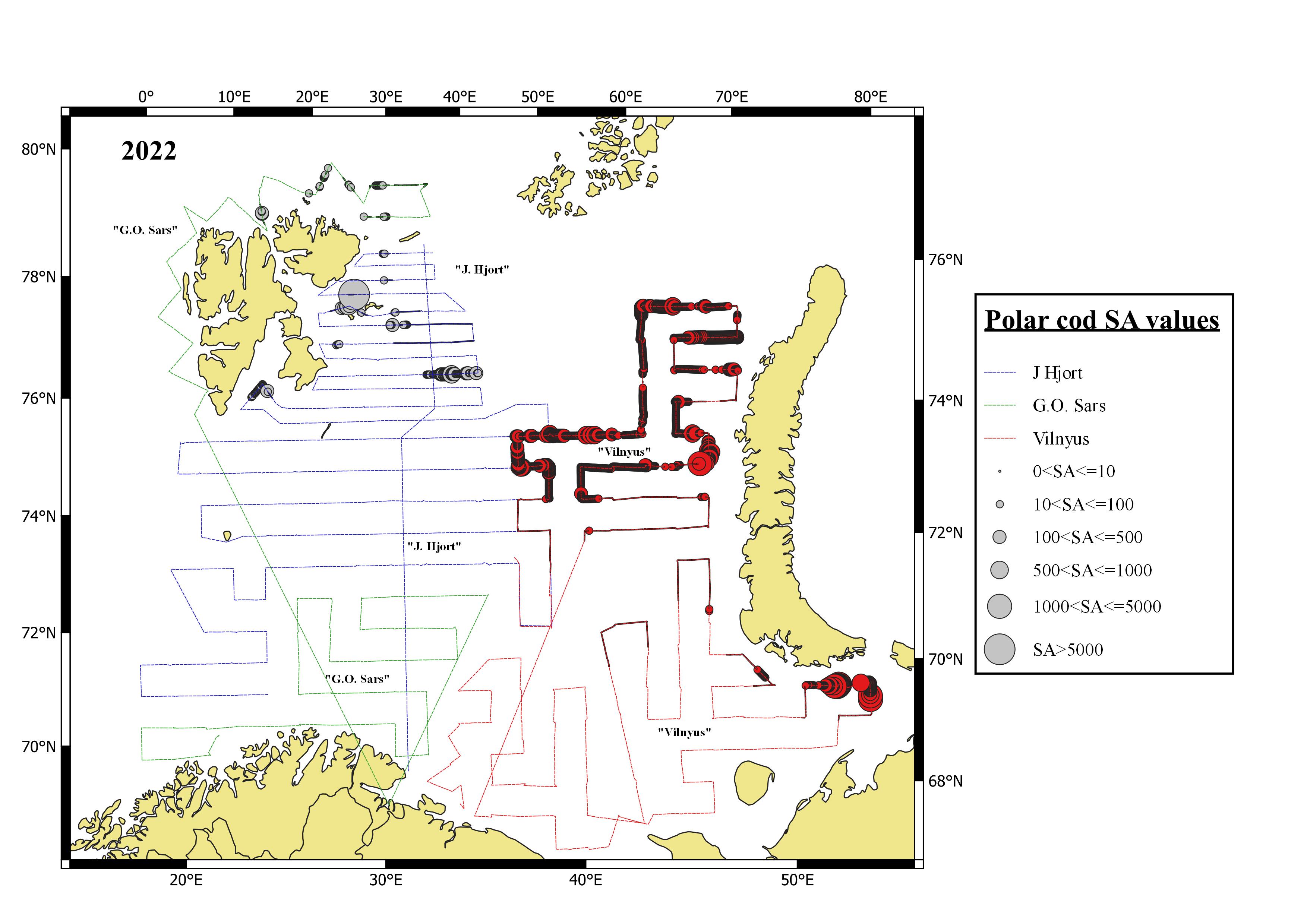
Only the western part of the Barents Sea was covered synoptically during BESS in 2022, the eastern part was covered late. The acoustic recordings of polar cod from both coverages are shown in Figure 7.2.1.1. There was very little polar cod observed in the west, the two significant concentrations were at 76°N close to the Russian border, and immediately north of Kong Karls land at ca. 77°N. In the eastern area, the polar cod had a wider distribution, although without very high concentrations. Polar cod was also recorded near the Kara Strait. The relatively low concentrations of polar cod this survey year contrast the wide area with polar cod aggregations from the previous two survey years.
7.2.2 Abundance estimation
Due to the incomplete coverage, no polar cod abundance estimation was done for 2022.
7.3 Herring (Clupea harengus)
7.3.1 Geographical distribution
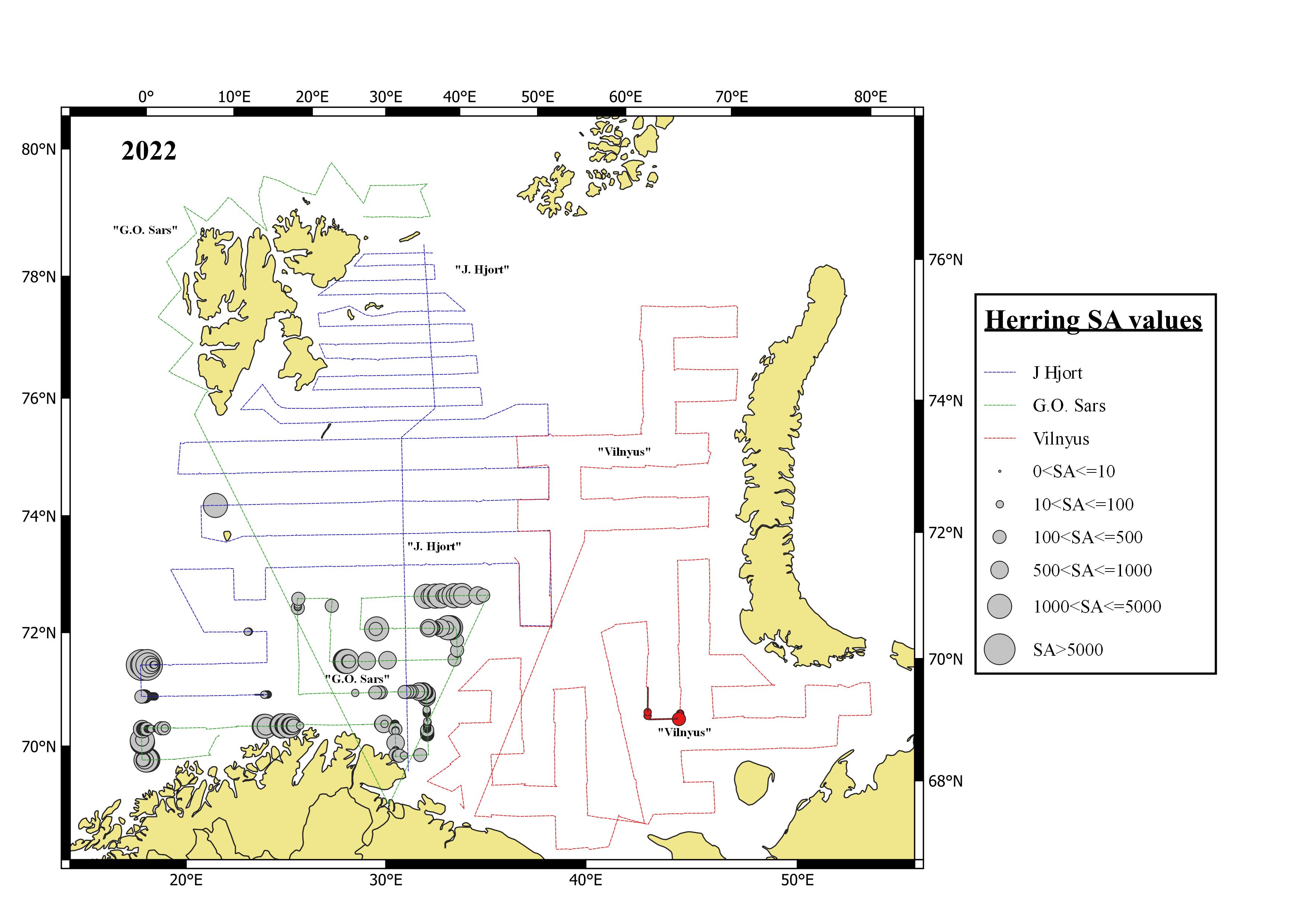
Only the Norwegian side of the Barents Sea was covered synoptically during BESS in 2022, the eastern part was covered late. The main distribution of young Norwegian spring spawning herring (NSSH) within the survey area was the North Cape bank around 30°E (Figure 7.3.1.1). In addition, there were concentrations of old fish (2016-yearclass) in the south-west. Very little herring was recorded during the late coverage in the east.
7.3.2 Abundance estimation
The estimated total number and biomass of NSSH in the Barents Sea in the autumn 2022 is shown in table 7.3.2.1, and the time series of abundance estimates is summarized in Table 7.3.2.2. Total numbers in 2022 was estimated at 6.78 billion individuals (Table 7.3.2.1). This is below the long-term average (Table 7.3.2.2). Abundance of all age groups were below the long-term average, and in particular the abundance of 3-year-olds was low as expected from the low number of 2-year-olds (2019 year-class) in the survey last year. 1-year-olds are dominating in abundance while the very strong 2016 year-class is still dominating the biomass estimate (Table 7.3.2.1).
|
Length (cm) |
Age/year class |
Sum (109) |
Biomass (103 t) |
Mean weight (g) |
||||
|
1 |
2 |
4 |
5 |
6 |
||||
|
2021 |
2020 |
2018 |
2017 |
2016 |
||||
|
13-14 |
0.000 |
|
|
|
|
0.000 |
0.005 |
20.00 |
|
14-15 |
0.001 |
|
|
|
|
0.001 |
0.014 |
19.33 |
|
15-16 |
1.436 |
|
|
|
|
1.436 |
32.311 |
22.50 |
|
16-17 |
0.639 |
|
|
|
|
0.639 |
19.994 |
31.31 |
|
17-18 |
1.116 |
|
|
|
|
1.116 |
44.951 |
40.27 |
|
18-19 |
1.058 |
0.049 |
|
|
|
1.107 |
49.944 |
45.11 |
|
19-20 |
0.148 |
0.134 |
|
|
|
0.282 |
15.186 |
53.76 |
|
20-21 |
0.045 |
|
|
|
|
0.045 |
2.499 |
56.00 |
|
21-22 |
|
0.027 |
|
|
|
0.027 |
2.016 |
76.00 |
|
22-23 |
|
0.009 |
|
|
|
0.009 |
0.743 |
84.00 |
|
23-24 |
|
0.448 |
|
|
|
0.448 |
36.567 |
81.58 |
|
24-25 |
|
|
|
|
|
0.000 |
|
|
|
25-26 |
|
0.215 |
|
|
|
0.215 |
27.592 |
128.16 |
|
26-27 |
|
|
|
0.009 |
|
0.009 |
1.273 |
144.00 |
|
27-28 |
|
|
0.009 |
|
|
0.009 |
1.326 |
150.00 |
|
28-29 |
|
|
|
|
|
0.000 |
|
|
|
29-30 |
|
|
0.352 |
|
|
0.352 |
78.041 |
221.50 |
|
30-31 |
|
|
0.037 |
|
0.008 |
0.045 |
11.978 |
263.73 |
|
31-32 |
|
|
|
0.120 |
0.084 |
0.204 |
57.812 |
283.82 |
|
32-33 |
|
|
0.091 |
0.183 |
0.251 |
0.526 |
159.025 |
302.48 |
|
33-34 |
|
|
|
0.008 |
0.074 |
0.083 |
26.189 |
317.15 |
|
34-35 |
|
|
|
|
0.231 |
0.231 |
76.631 |
331.43 |
|
35-36 |
|
|
|
|
|
0.000 |
1.602 |
388.00 |
|
TSN (109) |
4.442 |
0.882 |
0.490 |
0.320 |
0.649 |
6.783 |
|
|
|
TSB (103 t) |
155.248 |
76.574 |
117.268 |
92.468 |
202.539 |
|
645.699 |
|
|
Mean length (cm) |
16.54 |
22.53 |
29.60 |
31.49 |
32.67 |
|
|
|
|
Mean weight (g) |
34.95 |
86.78 |
239.44 |
289.16 |
312.03 |
|
|
94.95 |
Target strength estimation based on formula: TS= 20.0 log (L) – 71.9
|
Year |
Age 1 |
Age 2 |
Age 3 |
Age 4+ |
Total |
|||||
|
TSN |
TSB |
TSN |
TSB |
TSN |
TSB |
TSN |
TSB |
TSN |
TSB |
|
|
1999 |
48.759 |
716.0 |
0.986 |
31.0 |
0.051 |
2.0 |
|
|
49.795 |
749.0 |
|
2000 |
14.731 |
383.0 |
11.499 |
560.0 |
|
|
|
|
26.230 |
943.0 |
|
2001 |
0.525 |
12.0 |
10.544 |
604.0 |
1.714 |
160.0 |
|
|
12.783 |
776.0 |
|
2002 |
No data |
|
|
|
|
|
|
|
|
|
|
2003 |
99.786 |
3090.0 |
4.336 |
220.0 |
2.476 |
326.0 |
|
|
106.597 |
3636.0 |
|
2004 |
14.265 |
406.0 |
36.495 |
2725.0 |
0.901 |
107.0 |
|
|
51.717 |
3252.0 |
|
2005 |
46.380 |
984.0 |
16.167 |
1055.0 |
6.973 |
795.0 |
|
|
69.520 |
2833.0 |
|
2006 |
1.618 |
34.0 |
5.535 |
398.0 |
1.620 |
211.0 |
|
|
8.773 |
643.0 |
|
2007 |
3.941 |
148.0 |
2.595 |
218.0 |
6.378 |
810.0 |
0.250 |
46.0 |
13.164 |
1221.0 |
|
2008 |
0.030 |
1.0 |
1.626 |
77.0 |
3.987* |
287* |
3.223* |
373* |
8.866* |
738* |
|
2009 |
1.538 |
48.0 |
0.433 |
52.0 |
1.807 |
287.0 |
1.686 |
393.0 |
5.577 |
815.0 |
|
2010 |
1.047 |
35.0 |
0.315 |
34.0 |
0.234 |
37.0 |
0.428 |
104.0 |
2.025 |
207.0 |
|
2011 |
0.095 |
3.0 |
1.504 |
106.0 |
0.006 |
1.0 |
|
|
1.605 |
109.0 |
|
2012 |
2.031 |
36.0 |
1.078 |
66.0 |
1.285 |
195.0 |
|
|
4.394 |
296.0 |
|
2013 |
7.657 |
202.0 |
5.029 |
322.0 |
0.092 |
13.0 |
0.057 |
9.0 |
12.835 |
546.0 |
|
2014 |
4.188 |
62.0 |
1.822 |
126.0 |
6.825 |
842.0 |
0.162 |
25.0 |
13.011 |
1058.0 |
|
2015 |
1.183 |
6.0 |
9.023 |
530.0 |
3.214 |
285.0 |
0.149 |
24.0 |
13.569 |
845.0 |
|
2016 |
7.760 |
131.0 |
1.573 |
126.0 |
3.089 |
389.0 |
0.029 |
6.0 |
12.452 |
652.0 |
|
2017 |
34.950 |
820.0 |
2.138 |
141.0 |
3.465 |
412.0 |
0.982 |
210.0 |
41.537 |
1583.0 |
|
2018 |
No data |
|
|
|
|
|
|
|
|
|
|
2019 |
13.650 |
172.0 |
0.209 |
15.1 |
6.000 |
756.0 |
1.600 |
487.0 |
21.460 |
1430.0 |
|
2020 |
|
|
0.231 |
13.0 |
1.816 |
189.0 |
11.59* |
2796* |
13.636* |
2998* |
|
2021 |
1.410 |
80.8 |
0.120 |
10.1 |
0.360 |
39.5 |
0.720 |
144.7 |
2.610 |
275.1 |
|
2022** |
4.442 |
155.2 |
0.882 |
76.6 |
0.000 |
0.0 |
1.459 |
412.3 |
6.783 |
645.7 |
|
Average |
14.760 |
358.3 |
5.190 |
341.2 |
2.490 |
292.6 |
1.720 |
386.9 |
22.680 |
1193.2 |
*in mix with Kanin herring in the south-eastern part of the coverage area
**survey coverage only on Norwegian (western) side
7.4 Blue whiting (Micromesistius poutassou)
7.4.1 Geographical dirtribution
Blue whiting contributes to make up the mid-trophic pelagic component in the south-western part of the Barents Sea ecosystem. The Barents Sea is on the border of the distribution area for the blue whiting, but with incoming strong year-classes, increased abundance of young blue whiting in the Barents Sea is normally observed. During the 2022 survey, the westernmost parts of some transects were omitted due to reduction in effort (see Figure 7.4.1.1). These westernmost parts cover the shelf edge where blue whiting is typically distributed, and the cuts are likely to bias abundance of blue whiting downwards in comparison with previous years. The largest concentrations of blue whiting were found at the extreme south-western part of the survey area (Figure 7.4.1.1).
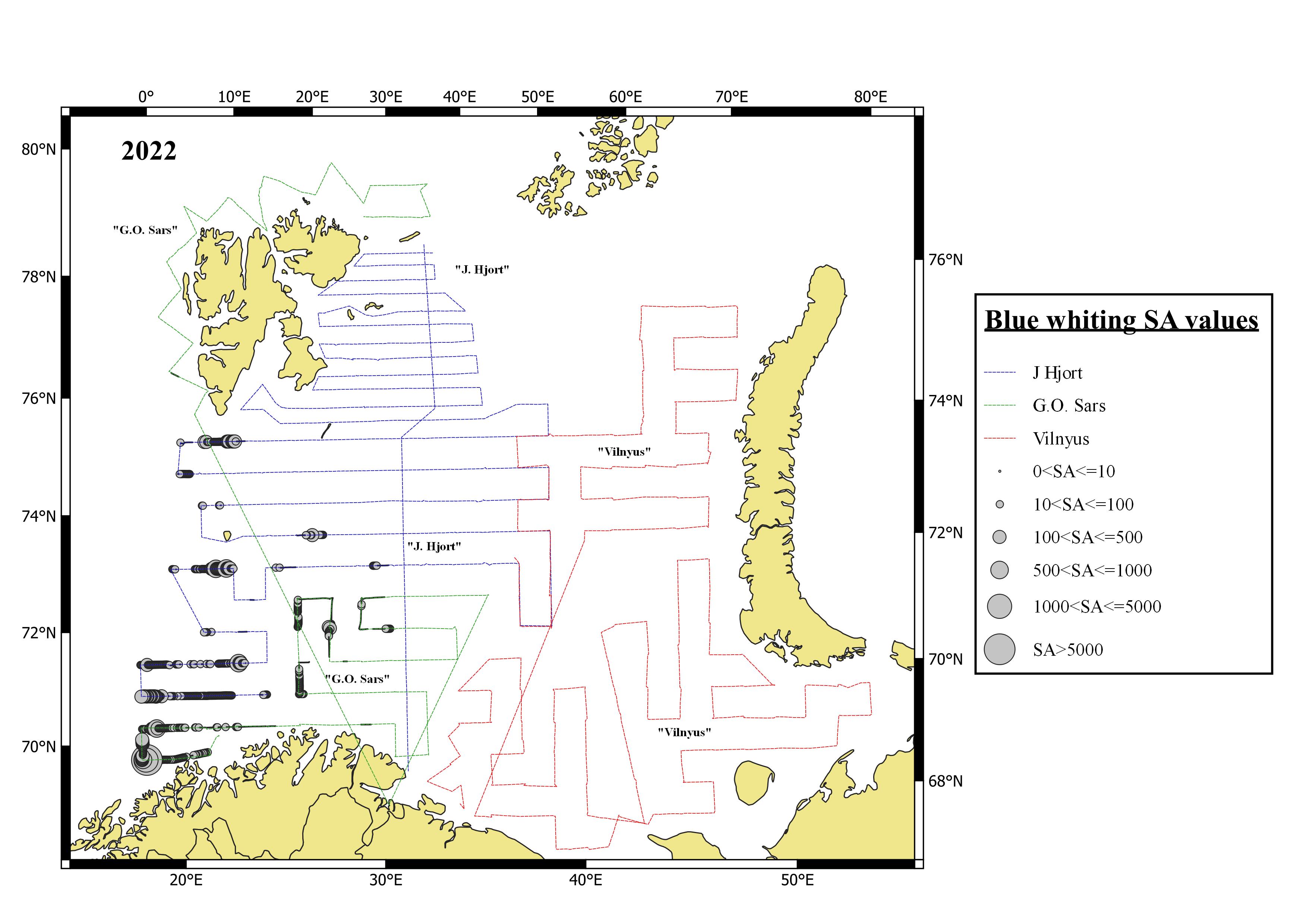
7.4.2 Abundance by size and age
The estimated total number and biomass of blue whiting in the Barents Sea in the autumn 2022 is shown in table 7.4.2.1, and the time series of abundance estimates is summarized in Table 7.4.2.2. Only data from the western coverage area are included in the estimate since the coverage in the east was late, but normally there is no blue whiting found in the east.
From 2004-2007 estimated biomass of blue whiting in the Barents Sea was between 200 000 and 350 000 tons (Table 7.4.2.2). In 2008 the estimated biomass dropped abruptly to only about 18% of the estimated biomass in the previous year, and it stayed low until 2012. From 2012 onwards it has been variable, but the last five years it has been lower than average despite that recruitment (abundance at age 1) in both 2021 and 2022 were high. This year estimated biomass was similar to the estimates from 2018, 2019 and last year (Table 7.4.2.3).
The 2021 year class (1-year olds) dominated in abundance while the 2020 year class (2-year-olds) dominated in biomass, but all age groups are below average in abundance (Table 7.4.2.1).
|
Length (cm) |
Age/year class |
Sum (106) |
Biomass (103 t) |
Mean weight (g) |
||||||||
|---|---|---|---|---|---|---|---|---|---|---|---|---|
|
1 |
2 |
3 |
4 |
5 |
6 |
7 |
8 |
10 |
||||
|
2021 |
2020 |
2019 |
2018 |
2017 |
2016 |
2015 |
2014 |
2012 |
||||
|
14-15 |
0.1 |
|
|
|
|
|
|
|
|
0.1 |
0.0 |
20.00 |
|
15-16 |
|
|
|
|
|
|
|
|
|
|
|
|
|
16-17 |
2.9 |
|
|
|
|
|
|
|
|
2.9 |
0.1 |
22.11 |
|
17-18 |
14.4 |
|
|
|
|
|
|
|
|
14.4 |
0.4 |
26.10 |
|
18-19 |
47.0 |
|
|
|
|
|
|
|
|
47.0 |
1.5 |
32.76 |
|
19-20 |
64.8 |
1.2 |
|
|
|
|
|
|
|
66.0 |
2.5 |
38.28 |
|
20-21 |
48.9 |
|
|
|
|
|
|
|
|
48.9 |
2.3 |
47.06 |
|
21-22 |
10.5 |
14.0 |
|
|
|
|
|
|
|
24.5 |
1.4 |
55.84 |
|
22-23 |
6.1 |
19.3 |
|
|
|
|
|
|
|
25.5 |
1.7 |
66.00 |
|
23-24 |
|
21.6 |
6.5 |
|
|
|
|
|
|
28.1 |
2.1 |
75.76 |
|
24-25 |
|
39.8 |
2.9 |
|
|
|
|
|
|
42.7 |
3.7 |
86.39 |
|
25-26 |
|
18.6 |
17.3 |
3.8 |
|
|
|
|
|
39.8 |
3.9 |
97.76 |
|
26-27 |
|
16.1 |
6.1 |
|
2.7 |
2.0 |
|
|
|
26.9 |
3.0 |
111.17 |
|
27-28 |
|
12.6 |
1.7 |
3.6 |
0.9 |
|
|
|
|
18.7 |
2.3 |
124.83 |
|
28-29 |
|
|
5.2 |
3.9 |
1.7 |
|
|
|
|
10.8 |
1.5 |
138.45 |
|
29-30 |
|
|
|
3.7 |
1.0 |
2.2 |
|
|
|
6.8 |
1.0 |
153.03 |
|
30-31 |
|
|
1.1 |
|
4.5 |
|
2.0 |
2.4 |
0.8 |
10.8 |
1.8 |
166.90 |
|
31-32 |
|
|
|
1.2 |
|
|
1.3 |
5.9 |
|
8.4 |
1.6 |
189.10 |
|
32-33 |
|
|
|
|
0.4 |
0.3 |
0.5 |
4.0 |
0.8 |
5.9 |
1.2 |
205.97 |
|
33-34 |
|
|
|
|
|
|
|
|
2.7 |
2.7 |
0.6 |
215.48 |
|
34-35 |
|
|
|
|
1.1 |
1.3 |
|
1.2 |
|
3.7 |
0.8 |
229.32 |
|
35-36 |
|
|
|
|
0.4 |
|
|
0.2 |
1.2 |
1.9 |
0.5 |
289.75 |
|
36-37 |
|
|
|
|
|
|
|
0.3 |
|
0.3 |
0.1 |
282.91 |
|
37-38 |
|
|
|
|
|
|
|
|
0.2 |
0.2 |
0.1 |
338.67 |
|
38-39 |
|
|
|
|
|
|
|
0.2 |
|
0.2 |
0.1 |
325.22 |
|
TSN (106) |
194.6 |
143.2 |
40.7 |
16.1 |
12.8 |
5.8 |
3.7 |
14.1 |
5.8 |
436.9 |
|
|
|
TSB (103 t) |
7.8 |
12.4 |
4.2 |
2.1 |
2.0 |
0.9 |
0.7 |
2.9 |
1.0 |
|
34.2 |
|
|
Mean length (cm) |
19.33 |
24.09 |
25.56 |
27.74 |
29.40 |
29.55 |
30.84 |
31.86 |
33.18 |
|
|
|
|
Mean weight (g) |
40.13 |
86.31 |
103.31 |
132.05 |
156.04 |
159.90 |
179.73 |
202.73 |
220.63 |
|
|
78.29 |
Target strength estimation based on formula: TS=20 log (L) - 65.2
Table 7.4.2.2 Blue whiting. Acoustic estimates by age in autumn 2004-2022. TSN and TSB are total stock numbers (106) and total stock biomass (103 tons) (only western coverage area included).
|
|
Age 1 |
Age 2 |
Age 3 |
Age 4+ |
Total |
|||||
|
TSN |
TSB |
TSN |
TSB |
TSN |
TSB |
TSN |
TSB |
TSN |
TSB |
|
|
2004 |
669 |
26 |
439 |
33 |
1056 |
98 |
1211 |
159 |
3575 |
327 |
|
2005 |
649 |
20 |
523 |
36 |
1051 |
86 |
809 |
102 |
3039 |
244 |
|
2006 |
47 |
2 |
478 |
34 |
730 |
70 |
922 |
129 |
2177 |
235 |
|
2007 |
+ |
+ |
116 |
11 |
892 |
92 |
743 |
107 |
1757 |
210 |
|
2008 |
+ |
+ |
+ |
+ |
10 |
1 |
238 |
36 |
247 |
37 |
|
2009 |
1 |
+ |
+ |
+ |
6 |
1 |
359 |
637 |
366 |
65 |
|
2010 |
|
|
2 |
|
5 |
1 |
155 |
31 |
163 |
33 |
|
2011 |
2 |
+ |
2 |
+ |
13 |
2 |
93 |
22 |
109 |
25 |
|
2012 |
583 |
27 |
64 |
8 |
58 |
9 |
321 |
77 |
1025 |
121 |
|
2013 |
1 |
|
349 |
28 |
135 |
13 |
175 |
42 |
664 |
84 |
|
2014 |
111 |
5 |
19 |
2 |
185 |
20 |
127 |
28 |
443 |
55 |
|
2015 |
1768 |
71 |
340 |
29 |
134 |
15 |
286 |
44 |
2529 |
159 |
|
2016 |
277 |
13 |
1224 |
82 |
588 |
48 |
216 |
36 |
2351 |
188 |
|
2017 |
43 |
2 |
253 |
22 |
503 |
49 |
269 |
38 |
1143 |
115 |
|
2018 |
|
|
18 |
1 |
74 |
8 |
215 |
29 |
332 |
40 |
|
2019 |
54 |
2 |
64 |
5 |
66 |
8 |
162 |
27 |
347 |
43 |
|
2020 |
110 |
5 |
19 |
2 |
11 |
1 |
56 |
11 |
196 |
18 |
|
2021 |
406 |
17 |
58 |
5 |
39 |
5 |
67 |
13 |
584 |
40 |
|
2022 |
195 |
8 |
143 |
12 |
41 |
4 |
58 |
10 |
437 |
34 |
|
Average |
328 |
16 |
242 |
21 |
295 |
28 |
341 |
83 |
1131 |
109 |
Target strength estimation based on formula: TS = 20 log (L) - 65.2 (Recalculation by Åge Høines, IMR 2017) Note:«+» <0.5
|
Year class |
Age |
Numbers (106) |
Mean weight (g) |
Biomass (103 t) |
||||
|
2021 |
2020 |
1 |
194.6 |
405.8 |
40.13 |
43.49 |
7.8 |
|
|
2020 |
2019 |
2 |
143.2 |
57.5 |
86.31 |
86.19 |
12.4 |
|
|
2019 |
2018 |
3 |
40.7 |
39.3 |
103.31 |
120.07 |
4.2 |
|
|
2018 |
2017 |
4+ |
58.4 |
67.0 |
169.04 |
190.70 |
9.6 |
|
|
Total stock in: |
|
|
|
|
|
|
|
|
|
2022 |
2021 |
Total |
436.9 |
583.9 |
78.38 |
69.26 |
34.2 |
|
8 - COMMERCIAL DEMERSAL FISH
Figures by: P. Krivosheya
In 2022 the eastern area was covered much later (covered 21/8-1/12) then the area covered by Norwegian vessels (16/8-4/10) so that the survey extended over a period of three and half months (see chapter 2). The lack of synoptic coverage and changes taking place during the survey period (e.g. migration between the western and the eastern part), may invalidate the results. The maps shown below should therefore be viewed with caution. Different colours show the surveyed areas in the Russian and Norwegian sectors.
Indices calculated from the ecosystem survey data are used in annual assessments of cod, haddock, the deep-water redfish and Greenland halibut. However, in 2023, the assessment-working group has to decide if the lack of synoptic coverage will make the indices too uncertain.
Data from the ecosystem survey is currently evaluated as part of the process of establishing an assessment model for the wolffish species.
Indices (number and biomass) calculated using Biofox for main bottom species except cod and haddock are presented in Table 8.1 and 8.2. Abundance indices by age based on the BESS data are used in annual assessments of cod (Gadus morhua) and haddock (Melanogrammus aeglefinus) and are given in Table 8.3 and 8.4.
|
Saithe |
Golden redfish |
Deep-water redfish |
Greenland halibut |
|||||
|
Year |
N |
B |
N |
B |
N |
B |
N |
B |
|
2004 |
36 |
40 |
13 |
9 |
263 |
104 |
182 |
39 |
|
2005 |
31 |
26 |
23 |
11 |
330 |
137 |
335 |
56 |
|
2006 |
28 |
49 |
16 |
16 |
526 |
219 |
430 |
77 |
|
2007 |
70 |
98 |
20 |
11 |
796 |
183 |
296 |
86 |
|
2008 |
3 |
7 |
42 |
17 |
864 |
96 |
153 |
76 |
|
2009 |
33 |
29 |
12 |
11 |
1003 |
213 |
191 |
90 |
|
2010 |
5 |
9 |
22 |
4 |
1076 |
112 |
186 |
150 |
|
2011 |
9 |
10 |
14 |
5 |
1271 |
105 |
175 |
88 |
|
2012 |
14 |
13 |
32 |
8 |
1587 |
196 |
209 |
86 |
|
2013 |
18 |
33 |
75 |
20 |
1608 |
256 |
160 |
94 |
|
2014 |
3 |
6 |
45 |
13 |
927 |
208 |
43 |
53 |
|
2015 |
105 |
153 |
9 |
5 |
894 |
214 |
79 |
52 |
|
2016 |
58 |
54 |
34 |
24 |
1527 |
319 |
82 |
40 |
|
2017 |
282 |
193 |
34 |
18 |
1705 |
212 |
134 |
74 |
|
2018* |
30 |
24 |
73 |
21 |
1298 |
260 |
||
|
2019 |
58 |
80 |
27 |
21 |
1126 |
313 |
166 |
61 |
|
2020 |
291 |
301 |
26 |
8 |
1086 |
291 |
276 |
55 |
|
2021 |
130 |
151 |
21 |
14 |
1701 |
191 |
141 |
56 |
|
2022 |
6 |
14 |
22 |
8 |
1257 |
231 |
558 |
142 |
|
Mean |
66 |
70 |
27 |
12 |
1086 |
200 |
211 |
76 |
|
Plaice |
Long rough dab |
Atlantic wolffish |
Spotted wolffish |
Northern wolffish |
||||||
|
Year |
N |
B |
N |
B |
N |
B |
N |
B |
N |
B |
|
2004 |
53 |
43 |
2951 |
306 |
15 |
7 |
12 |
31 |
3 |
26 |
|
2005 |
19 |
11 |
2753 |
272 |
16 |
6 |
11 |
26 |
3 |
26 |
|
2006 |
36 |
19 |
3705 |
378 |
26 |
11 |
12 |
46 |
2 |
19 |
|
2007 |
120 |
55 |
5327 |
505 |
42 |
11 |
12 |
42 |
3 |
25 |
|
2008 |
57 |
29 |
3942 |
477 |
25 |
14 |
13 |
51 |
3 |
22 |
|
2009 |
21 |
13 |
2600 |
299 |
20 |
8 |
9 |
47 |
3 |
31 |
|
2010 |
34 |
21 |
2520 |
356 |
17 |
17 |
7 |
37 |
3 |
25 |
|
2011 |
36 |
26 |
2507 |
322 |
20 |
13 |
9 |
47 |
6 |
42 |
|
2012 |
21 |
13 |
4563 |
584 |
22 |
9 |
13 |
83 |
8 |
45 |
|
2013 |
36 |
29 |
4932 |
565 |
27 |
30 |
13 |
84 |
12 |
52 |
|
2014 |
170 |
121 |
3046 |
413 |
12 |
12 |
8 |
51 |
6 |
34 |
|
2015 |
107 |
79 |
3624 |
438 |
33 |
37 |
12 |
86 |
9 |
63 |
|
2016 |
37 |
29 |
3369 |
402 |
40 |
24 |
13 |
40 |
8 |
51 |
|
2017 |
17 |
19 |
4604 |
538 |
30 |
29 |
14 |
63 |
8 |
63 |
|
2018* |
||||||||||
|
2019 |
146 |
101 |
3627 |
472 |
37 |
20 |
15 |
51 |
13 |
76 |
|
2020 |
94 |
37 |
3443 |
454 |
44 |
27 |
22 |
55 |
13 |
65 |
|
2021 |
195 |
106 |
3688 |
396 |
42 |
28 |
17 |
37 |
7 |
59 |
|
2022 |
242 |
109 |
3734 |
404 |
24 |
20 |
9 |
49 |
5 |
40 |
|
Mean |
80 |
48 |
3608 |
421 |
27 |
18 |
12 |
51 |
6 |
42 |
| Year/age | 1 | 2 | 3 | 4 | 5 | 6 | 7 | 8 | 9 | 10 | 11 | 12+ |
| 2004 | 330.6 | 329.7 | 147.7 | 421.5 | 150.2 | 79.8 | 40.2 | 10.1 | 2.2 | 0.5 | 0.1 | 0.2 |
| 2005 | 440.7 | 146.6 | 216.6 | 55.8 | 100.9 | 28.0 | 15.6 | 5.7 | 1.2 | 0.5 | 0.1 | 0.1 |
| 2006 | 479.0 | 509.7 | 186.1 | 205.6 | 59.9 | 69.8 | 17.6 | 8.1 | 2.6 | 0.6 | 0.2 | 0.0 |
| 2007 | 333.3 | 505.4 | 586.2 | 159.2 | 79.1 | 24.6 | 26.9 | 6.0 | 2.2 | 0.9 | 0.1 | 0.2 |
| 2008 | 130.9 | 372.6 | 652.6 | 483.4 | 132.3 | 51.1 | 12.8 | 17.5 | 3.3 | 0.9 | 0.2 | 0.4 |
| 2009 | 569.7 | 93.5 | 202.3 | 280.6 | 289.6 | 101.7 | 31.9 | 12.7 | 7.3 | 2.6 | 0.8 | 0.5 |
| 2010 | 310.3 | 84.2 | 56.8 | 177.0 | 397.2 | 424.9 | 142.7 | 38.5 | 10.5 | 6.8 | 1.6 | 0.6 |
| 2011 | 509.8 | 160.0 | 123.6 | 101.5 | 240.2 | 300.4 | 178.4 | 32.3 | 7.7 | 1.8 | 1.3 | 0.9 |
| 2012 | 1454.3 | 255.9 | 229.1 | 146.4 | 70.0 | 150.8 | 165.2 | 84.5 | 12.7 | 4.4 | 1.6 | 2.1 |
| 2013 | 914.2 | 659.0 | 249.1 | 183.6 | 125.7 | 63.2 | 118.2 | 130.2 | 53.8 | 9.1 | 3.3 | 2.5 |
| 2014 | 308.2 | 155.1 | 190.0 | 108.6 | 93.9 | 52.8 | 30.4 | 50.2 | 36.3 | 12.1 | 3.4 | 2.4 |
| 2014 * | 339.0 | 184.0 | 226.3 | 122.2 | 103.4 | 67.7 | 42.1 | 81.3 | 78.9 | 28.1 | 4.7 | 2.8 |
| 2015 | 725.3 | 154.0 | 174.4 | 225.2 | 141.3 | 72.6 | 48.6 | 26.2 | 35.3 | 26.6 | 7.9 | 2.7 |
| 2016 | 350.8 | 341.3 | 77.2 | 93.7 | 121.6 | 70.1 | 44.4 | 27.2 | 13.8 | 13.2 | 5.4 | 3.0 |
| 2017 | 757.5 | 260.6 | 375.0 | 141.5 | 104.9 | 120.9 | 62.6 | 28.0 | 11.2 | 6.4 | 4.4 | 7.2 |
| 2018* | 2100.3 | 413.8 | 183.6 | 148.9 | 60.0 | 37.6 | 57.1 | 20.2 | 14.4 | 5.8 | 3.6 | 6.3 |
| 2019 | 560.2 | 475.2 | 416.6 | 232.3 | 215.1 | 76.6 | 42.2 | 44.4 | 16.1 | 4.9 | 2.2 | 2.9 |
| 2020 | 66.5 | 104.7 | 133.7 | 134.3 | 98.6 | 79.6 | 31.6 | 15.7 | 11.4 | 2.9 | 1.1 | 1.1 |
| 2021 | 61.2 | 51.8 | 84.0 | 100.0 | 80.3 | 46.2 | 33.6 | 12.5 | 4.7 | 5.0 | 2.4 | 1.4 |
| 2022 | 214.0 | 39.2 | 25.5 | 32.8 | 34.4 | 33.7 | 18.5 | 9.8 | 2.5 | 0.8 | 0.5 | 0.3 |
| Year/age | 1 | 2 | 3 | 4 | 5 | 6 | 7 | 8 | 9 | 10 | 11 | 12+ |
| 2004 | 189.0 | 268.5 | 123.4 | 70.3 | 69.1 | 31.5 | 3.0 | 1.7 | 0.0 | 0.1 | 0.0 | 0.1 |
| 2005 | 603.8 | 114.2 | 324.6 | 89.5 | 30.4 | 32.2 | 15.0 | 0.5 | 0.7 | 0.2 | 0.1 | 0.2 |
| 2006 | 2270.2 | 929.1 | 107.5 | 124.6 | 41.6 | 19.0 | 17.5 | 7.3 | 0.8 | 0.5 | 0.1 | 0.1 |
| 2007 | 988.4 | 1818.9 | 1282.9 | 88.5 | 90.4 | 19.2 | 5.9 | 7.1 | 1.9 | 0.9 | 0.2 | 0.2 |
| 2008 | 322.0 | 1291.9 | 1154.9 | 406.0 | 43.1 | 35.5 | 4.9 | 2.5 | 2.3 | 0.3 | 0.0 | 0.0 |
| 2009 | 134.8 | 143.8 | 650.7 | 619.1 | 305.9 | 21.0 | 6.5 | 0.9 | 0.5 | 0.0 | 0.0 | 0.0 |
| 2010 | 274.4 | 65.1 | 184.0 | 865.3 | 666.4 | 147.7 | 15.8 | 2.7 | 0.0 | 0.1 | 0.1 | 0.3 |
| 2011 | 105.3 | 113.6 | 40.4 | 73.8 | 392.9 | 301.4 | 37.4 | 3.0 | 0.3 | 0.1 | 0.0 | 0.2 |
| 2012 | 591.1 | 41.5 | 92.5 | 20.3 | 67.6 | 214.1 | 152.0 | 12.7 | 0.3 | 0.2 | 0.0 | 1.5 |
| 2013 | 155.9 | 223.0 | 25.8 | 65.2 | 19.6 | 50.8 | 150.1 | 76.4 | 7.0 | 0.4 | 0.0 | 0.2 |
| 2014 | 264.8 | 75.1 | 261.6 | 40.8 | 70.2 | 25.8 | 60.5 | 85.8 | 18 | 1.4 | 0.2 | 0.0 |
| 2015 | 320.0 | 145.2 | 42.1 | 213.6 | 25.1 | 37.1 | 20.6 | 47.9 | 33.8 | 8.6 | 0.2 | 0.2 |
| 2016 | 793.8 | 144.9 | 209.3 | 34.4 | 184.1 | 48.0 | 56.8 | 40.4 | 65.8 | 47.5 | 11.8 | 0.9 |
| 2017 | 935.8 | 189.3 | 70.3 | 70.3 | 11.5 | 20.5 | 4.0 | 4.0 | 5.4 | 4.4 | 4.8 | 0.7 |
| 2018* | ||||||||||||
| 2019 | 379.4 | 585.3 | 897.0 | 160.7 | 38.1 | 15.1 | 5.3 | 5.0 | 1.9 | 2.1 | 2.1 | 5.6 |
| 2020 | 26.8 | 57.8 | 204.1 | 341.4 | 58.8 | 4.9 | 2.0 | 0.8 | 0.2 | 0.7 | 0.1 | 0.5 |
| 2021 | 107.8 | 35.9 | 129.6 | 346.8 | 329.0 | 32.3 | 5.4 | 0.9 | 0.3 | 0.6 | 0.4 | 0.1 |
| 2022 | 690.2 | 106.6 | 18.7 | 59.4 | 84.6 | 80.2 | 9.5 | 2.2 | 0.0 | 0.0 | 0.2 | 0.0 |
8.1 Cod (Gadus morhua)
At the time of survey cod usually reaches the northern and eastern limits of its feeding area. In general, the cod was distributed almost over the entire area surveyed (Fig. 8.1) .
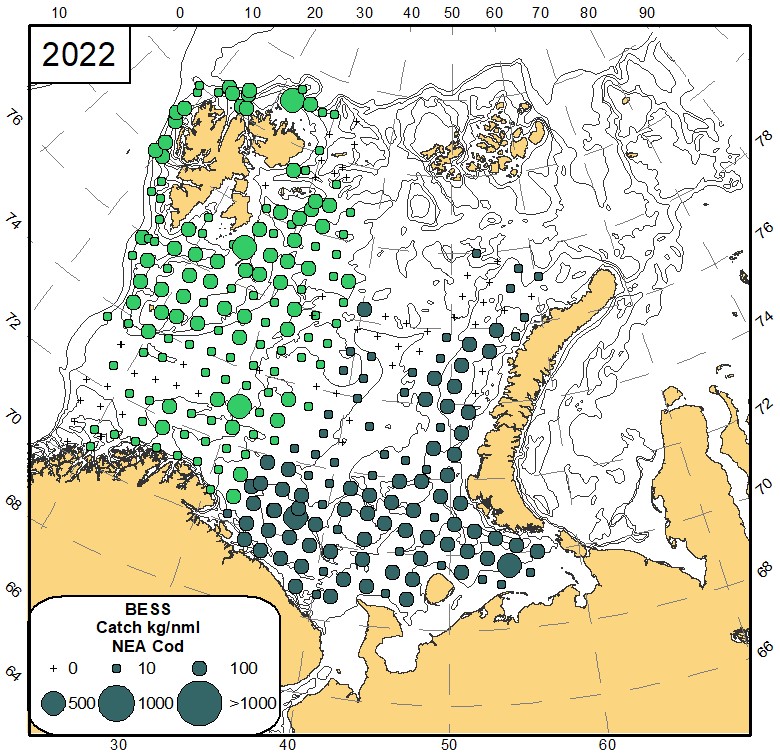
8.2 Haddock (Melanogrammus aeglefinus)
Main concentrations of haddock were found along the along Finnmark and Murman coasts, and in the south-eastern Barents Sea (Fig.8.2).
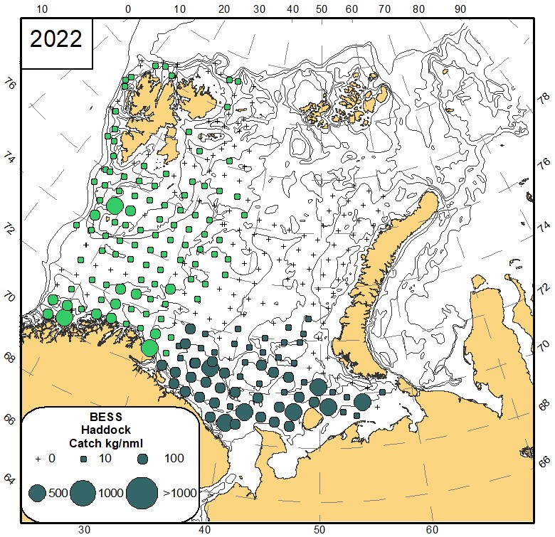
8.3 Saithe (Pollachius virens)
The ecosystem survey only covers a small part of the distribution of saithe and the data is not used for stock assessment. As in previous years, the highest catches were in the south west and along the Norwegian coast (Fig.8.3).
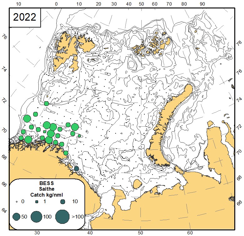
8.4 Greenland halibut (Reinhardtius hippoglossoides)
BESS covers mainly an area where young Greenland halibut is found, including nursery aresa in the northernmost part. However, in recent years larger Greenland halibut has increasingly been registered in the deep-water central parts of Barents Sea. This affects the stock indices when expressed in biomass. The BESS registrations are divided into northern (nursery) areas and southern part. Thus, two indices are estimated, each of them additionally divided by sex, based on BESS. Moreover two trawl indices from surveys that cover deeper waters than BESS, at the continental slope, are also used.
As in previous years, the Greenland halibut was observed in almost all catches in the deep areas of the Barents Sea (Fig. 8.4). Compared to last year the distribution pattern was similar. The main concentrations of G. halibut were observed around Svalbard (Spitsbergen), to the west of Franz Josef Land, and in the Bear Island Trench. Noticeably there were substantial registrations of G. halibut in an area towards the Yermak Plateau that has not been covered in previous surveys.
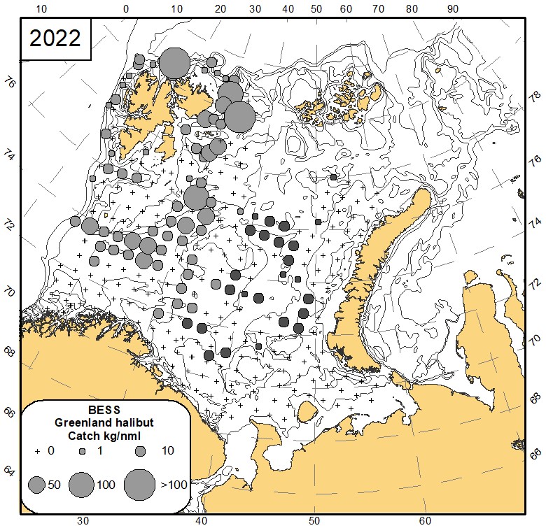
8.5 Golden redfish (Sebastes norvegicus)
Data from the ecosystem survey is not used in the assessment of golden redfish. In 2022, centres of abundance for golden redfish were observed along the coast of the Troms region in Norway and along the Murman coast, with the highest catches in the latter region (Fig. 8.5). The distribution north and west of Svalbard was very similar to 2021 and as in earlier years observations in the eastern Barents Sea, were few and of low abundance.
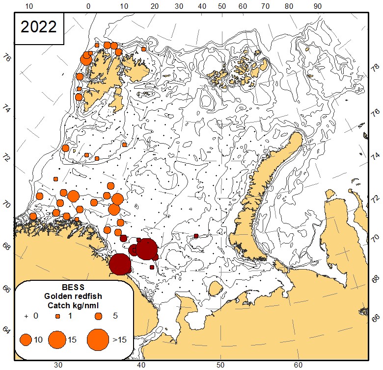
8.6 Deep-water redfish (Sebastes mentella)
Data from BESS are used in the assessment of deep-water redfish. As in previous years, deep-water redfish were only absent from an area north of Bear Island and in the south-eastern part of the Barents Sea. (Fig. 8.6). Highest catches of deep-water redfish were concentrated in the area south and southeast of Bear Island, particularly along the Bear Island Trench. Likewise high catches were recorded along the shelf break north of Bear Island and up to Svalbard. Catch weight decreased towards the eastern Barents Sea.
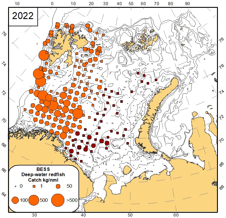
8.7 Long rough dab (Hippoglossoides platessoides)
As usual, long rough dab were found in the entire area surveyed (Fig. 8.7). The highest catches were in the northern part of the surveyed area along the slopes of the Svalbard and Central Banks.
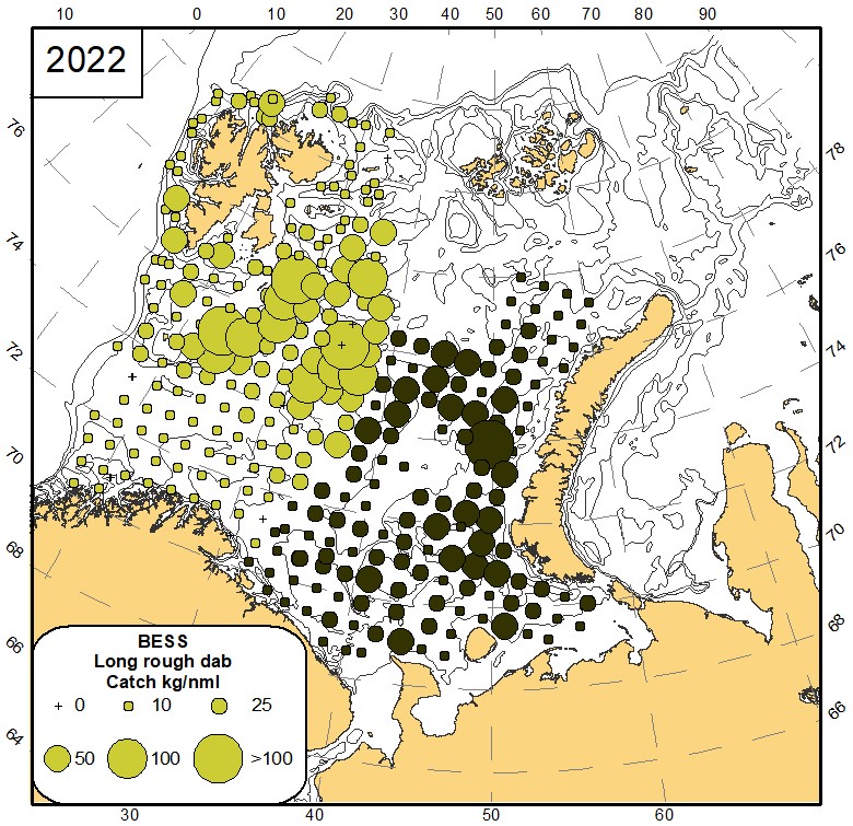
8.8 Plaice (Pleuronectes platessa)
Plaice is mainly found in the southeastern Barents Sea. In 2022 almost the entire distribution area of plaice was covered (Fig. 8.8).
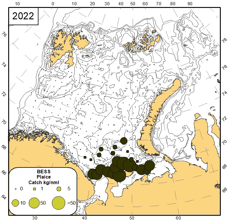
8.9 Atlantic wolffish (Anarhichas lupus)
Atlantic wolffish is the most numerous of the three species of wolffishes inhabiting the Barents Sea, while due to its smaller size has the lowest biomass of the three species. Atlantic wolffish was mainly found in Atlantic water along the western coast of Svalbard (Fig. 8.9).
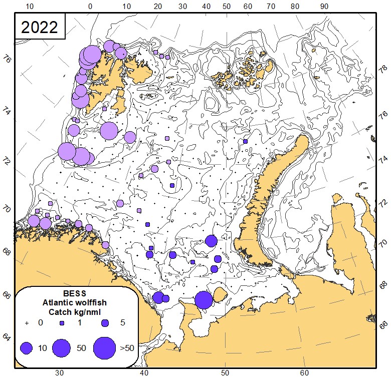
8.10 Spotted wolffish (Anarhichas minor)
In 2020 the spotted wolffish was found along the slopes of the Svalbard and Central Banks (Fig. 8.10).
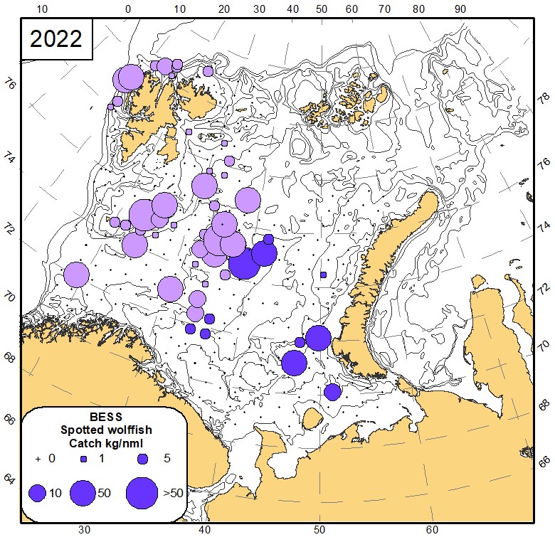
8.11 Northern wolffish (Anarhichas denticulatus)
In 2022 Northern wolffish was distributed along the slopes of west of Svalbard, along the slopes of Hopen Trench extending into the slopes of the Central Basin in the eastern Barents Sea (Fig. 8.11).
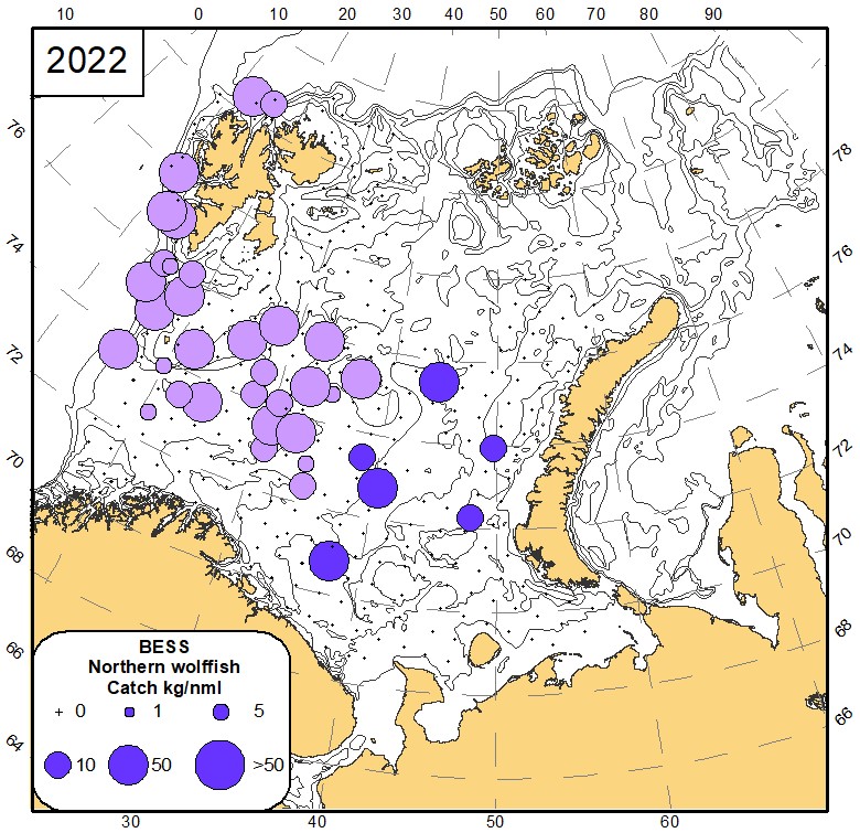
9 - FISH BIODIVERSITY
9.1 Small non-target fish species
Text: Elena Eriksen
The small non-target fish species from the BESS 2022 survey will not be ready for publication in this report. The data will be included in the BESS 2023 survey report.
9.2 Fish biodiversity in the demersal compartment
by Tatiana Prokhorova, Edda Johannesen, Andrej Dolgov, Rupert Wienerroither and Pavel Krivosheya
Figures by P. Krivosheya
Norway pout (Trisopterus esmarkii). Norway pout is usually found in the western part of the ecosystem survey area, and as in the previous years the highest concentrations in 2022 were found in the Norwegian part of the area (Fig. 9.2.1). Thus, the results on the distribution of this species in 2022 is likely hardly impacted by the time differences in survey coverage in the eastern and western Barents Sea.
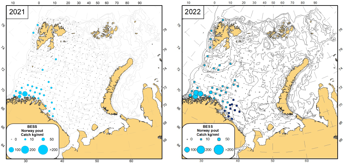
Norway redfish (Sebastes viviparus). Norway redfish is usually found in the southwestern part of the surveyed area. Thus, the results for this species are less impacted by the gap in research time between the Russian and Norwegian zones than species with a wider distribution.
In 2022 Norway redfish was distributed approximately in the same area as in 2021 (Fig. 9.2.2). The main concentrations of this species occurred in the south-western area of the survey along the Norwegian coast.
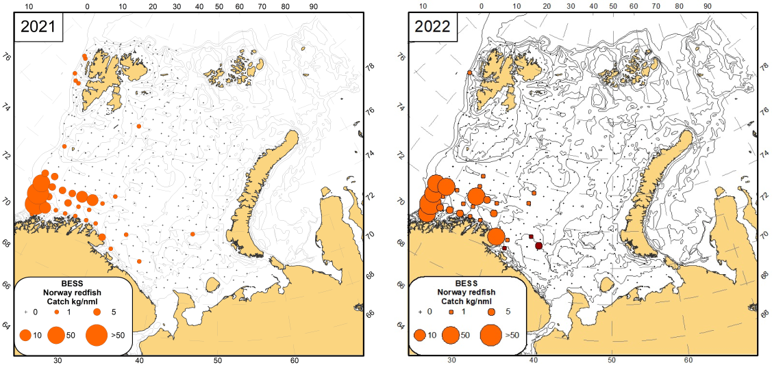
Thorny skate (Amblyraja radiata) and Arctic skate (Amblyraja hyperborea) were selected as indicator species to study how ecologically similar fishes from different zoogeographic groups respond to changes of their environment. Thorny skate belongs to the mainly boreal zoogeographic group and is widely distributed in the Barents Sea except the most north-eastern areas, while Arctic skate belongs to the Arctic zoogeographic group and is distributed in the cold waters of the northern area.
In 2022 thorny skate was distributed in a wide area from the north-western to the south-western and south-eastern Barents Sea where warm Atlantic and Coastal Waters dominated (Figure 9.2.3).

Only one specimen of Arctic skate was observed in 2022 (compared to six stations in 2021), (Figure 9.2.4). It was found in 157 m depth.
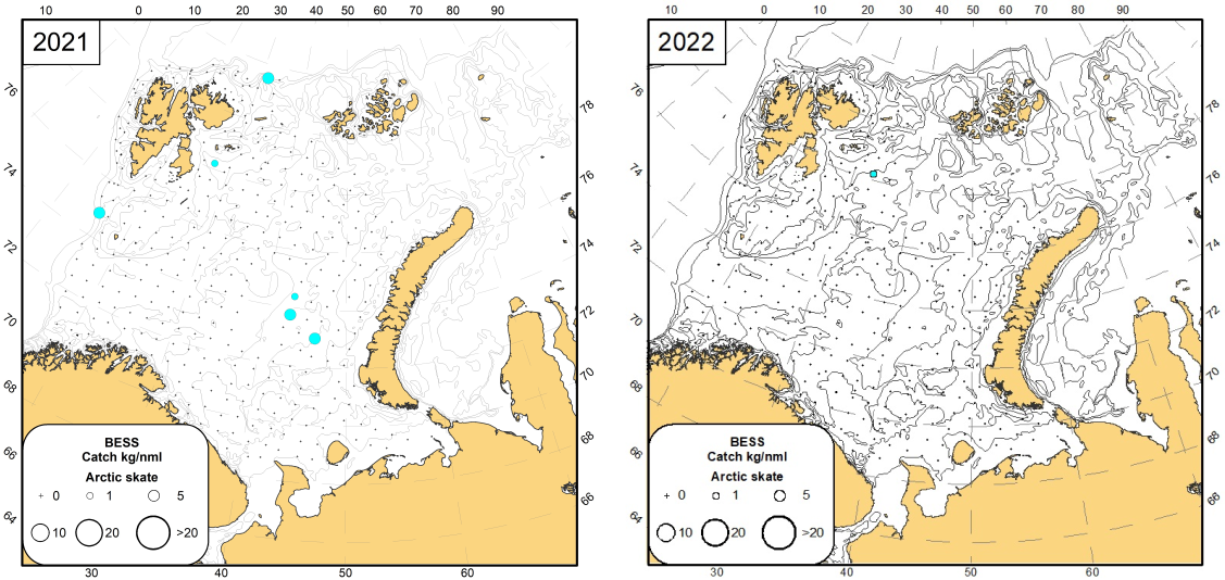
9.3 Uncommon or rare species
Text by Tatiana Prokhorova, Edda Johannesen, Andrei Dolgov, Rupert Wienerroither and Pavel Krivosheya
Figures by P. Krivosheya
Rare or uncommon species are either species that are not caught at the Barents Sea ecosystem survey every year, or caught most years but in low numbers and with limited occurrence. Most of these species usually occur in areas adjacent to the Barents Sea and were therefore found mainly along the border of the surveyed area. Some uncommon species were also observed in the Barents Sea during the ecosystem survey in 2022 (Figure 9.3.1).
For example, hooknose Agonus cataphractus known in coastal waters of the eastern North Atlantic and the adjacent Arctic from the British Isles northward to the southern Barents Sea and the White Sea, within the temperature range 4-12 °C (Wienerroither et al., 2011; Mecklenburg et al., 2018). During the survey 15 individuals of this species were found on 2 stations in the shallow regions in the south-eastern area of the survey (Figure 9.3.1). Hooknose was observed at 24-33 m depth and bottom temperature 3.3-3.9 °C in 2022.
Arctic rockling Gaidropsarus argentatus is known from off southern Greenland, off Iceland and the Faroe Islands to the Norwegian coast and northward to the Barents Sea (Wienerroither et al., 2011; Mecklenburg et al., 2018). This species usually lives at depths below 500 m and prefers low temperature (around 0 °C). Accordingly, during the survey 2 individuals of this species were found on 2 stations in deepwater areas in the north (at 526 m depth) and west (at 461 m depth) of the Barents Sea (Figure 9.3.1).
Arctic lamprey Lethenteron camtschaticum is an anadromous species known from northeastern Norway eastward to the Bering Sea, and the northwestern Pacific Ocean (Wienerroither et al., 2011. This species usually lives near the coast, but can also be found in open areas of the sea in the upper layers (Dolgov et al., 2018). This species parasitizes on various marine and freshwater fishes and is rather rare to observe. Despite Arctic lamprey was found in the southeastern part of the surveyed area only in previous years, it was found in the central part in 2022 (Figure 9.3.1).
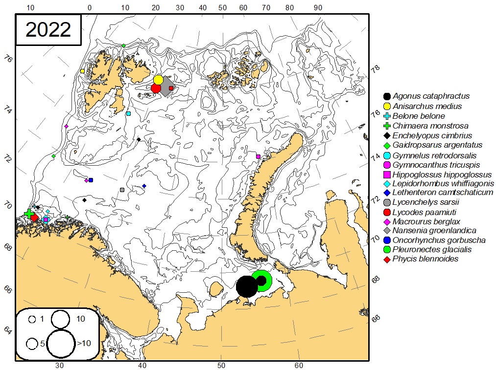
9.4 Zoogeographic groups
Text by Tatiana Prokhorova, Edda Johannesen, Andrej Dolgov, Rupert Wienerroither and Pavel Krivosheya
Figures by P. Krivosheya
During the 2022 ecosystem survey in total 85 fish species from 31 families were recorded in the catches, and some specimens were only identified to genus or family level. The highest number of species were found in the families Zoarcidae (12 species), Cottidae, Gadidae, and Pleuronectidae (8 species each). All recorded species belonged to the 7 zoogeographic groups: widely distributed, south boreal, boreal, mainly boreal, Arctic-boreal, mainly Arctic and Arctic as defined by Andriashev and Chernova (1994). Mecklenburg et al. (2018) in the recent “Marine Fishes of the Arctic Region” reclassified some of the species and the zoogeographic categorisation comprises six groups: widely distributed, boreal, mainly boreal, Arctic- boreal, mainly Arctic and Arctic. We use Andriashev and Chernova classification here due to the lack of comparative studies of the old and new classification applied to the Barents Sea. Only bottom trawl data were used, and only non-commercial species were included into the analysis, both demersal (including bentho-pelagic) and pelagic (neritopelagic, epipelagic, bathypelagic) species (Andriashev and Chernova, 1994, Parin, 1968, 1988). Among the analyzed species most belong to the Arctic (27.1 %), mainly boreal (27.1 %), and boreal (22.0 %) zoogeographic groups.
Widely distributed (only ribbon barracudina Arctozenus risso represents this group), south boreal (e.g. grey gurnard Eutrigla gurnardus, silvery pout Gadiculus argenteus, greater forkbeard Phycis blennoides) and boreal (e.g. lemon sole Microstomus kitt, stout eelblenny Anisarchus medius, silvery lightfish Maurolicus muelleri) species were mostly found in the central, southwestern and western part of the survey area where warm Atlantic and Coastal Waters dominate (Figure 9.4.1).
Mainly boreal species (e.g. lesser sandeel Ammodytes marinus, snakeblenny Lumpenus lampretaeformis, greater eelpout Lycodes esmarkii) were widely found throughout the survey area (Figure 9.2.1).
Arctic-boreal species (e.g. Atlantic poacher Leptagonus decagonus, ribbed sculpin Triglops pingelii) were found in the central and northern part of the Barents Sea (Figure 9.4.1).
Mainly Arctic (e.g. Arctic flounder Liopsetta glacialis, Atlantic spiny lumpsucker Eumicrotremus spinosus, slender eelblenny Lumpenus fabricii) and Arctic (e.g. Arctic alligatorfish Aspidophoroides olrikii, pale eelpout Lycodes pallidus, leatherfin lumpsucker Eumicrotremus derjugini) species were mainly found on the northern part of the Barents Sea (Figure 9.4.1). Species of these groups mostly occur in areas influenced by cold Arctic Water, Spitsbergen Bank Water and Novaya Zemlya Coastal Water.
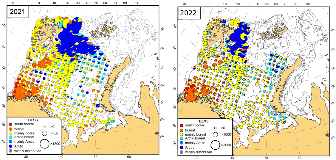
References
Dolgov, A.V., A.P. Novoselov, T.A. Prokhorova, G.V. Fuks, D.V. Prozorkevich, N.V. Chernova, V.S. Sherstkov, A.L. Levitskiy. Atlas of the Kara Sea fish. – Murmansk: PINRO, 2018. – 271 pp. (in Russian)
Mecklenburg, C.W., A. Lynghammar, E. Johannesen, I. Byrkjedal. J.S. Christiansen, A.V. Dolgov, O.V. Karamushko, T.A. Mecklenburg, P.R. Møller, D. Steinke, and R.M. Wienerroither. 2018. Marine Fishes of the Arctic Region. Conservation of Arctic Flora and Fauna, Akureyri, Iceland.
Wienerroither R., Johannesen E., Dolgov A., Byrkjedal I., Bjelland O., Drevetnyak K., Eriksen K.B., Høines Å., Langhelle G., Langøy H., Prokhorova T., Prozorkevich D., Wenneck T. Atlas of the Barents Sea fishes. IMR/PINRO Joint Report Series, No. 1/2011. – 272 pp.
10 - COMMERCIAL SHELLFISH
10.1 Northern shrimp (Pandalus borealis)
Text by: Sergei Bakanev and Carsten Hvingel
Figures by: J. Zhak
During the survey in 2022 293 trawl hauls were completed – 246 of them contained northern shrimp. The biomass of shrimp varied from several grams to 244.8 kg/nm with an average catch of 6.6±1.0 kg nm (Table 10.1.1). Average values are reported with standard error (SEM).
Table 10.1.1. The catch characteristics of the Northern shrimp (include SEM) during BESS in 2005-2022.
|
Year |
Total number of station |
Number of station with shrimp |
Mean catch, ind./nml |
Mean catch, kg/nml |
|
2005 |
224 |
169 |
856.3±12.1 |
12.1±4.3 |
|
2006 |
637 |
480 |
3460.8±21.4 |
15.0±0.9 |
|
2007 |
551 |
426 |
2875.5±19.7 |
13.2±0.9 |
|
2008 |
431 |
329 |
1846.6±17.7 |
9.2±0.7 |
|
2009 |
378 |
310 |
1673.0±17.4 |
7.9±0.9 |
|
2010 |
319 |
238 |
2625.5±15.3 |
12.0±1.2 |
|
2011 |
391 |
304 |
2165.2±17.2 |
10.4±0.9 |
|
2012 |
443 |
325 |
2351.2±18.0 |
12.0±1.0 |
|
2013 |
487 |
388 |
1838.2±19.1 |
9.5±0.6 |
|
2014 |
165 |
101 |
1676.0±10.1 |
8.4±1.0 |
|
2015 |
334 |
247 |
1371.0±15.6 |
7.1±0.6 |
|
2016 |
317 |
187 |
1457.9±13.1 |
7.0±0.6 |
|
2017 |
339 |
281 |
2021.4±16.3 |
13.8±1.9 |
|
2018 |
217 |
160 |
1759.0±11.9 |
10.2±1.4 |
|
2019 |
323 |
254 |
1577.5±3.1 |
9.1±0.2 |
|
2020 |
461 |
317 |
717.2±77.3 |
4.6±0.4 |
|
2021 |
341 |
275 |
1487.4±68.2 |
7.8±0.4 |
|
2022 |
293 |
246 |
1175.8±177.4 |
6.6±1.0 |
|
Total |
7064 |
5154 |
1417.5±42.6 |
8.1±0.2 |
As in previous years the densest concentrations of shrimp in 2022 were registered in central part of the Barents Sea, around Svalbard (Spitsbergen) and in the Franz Victoria Trough (Fig. 10.1.1).
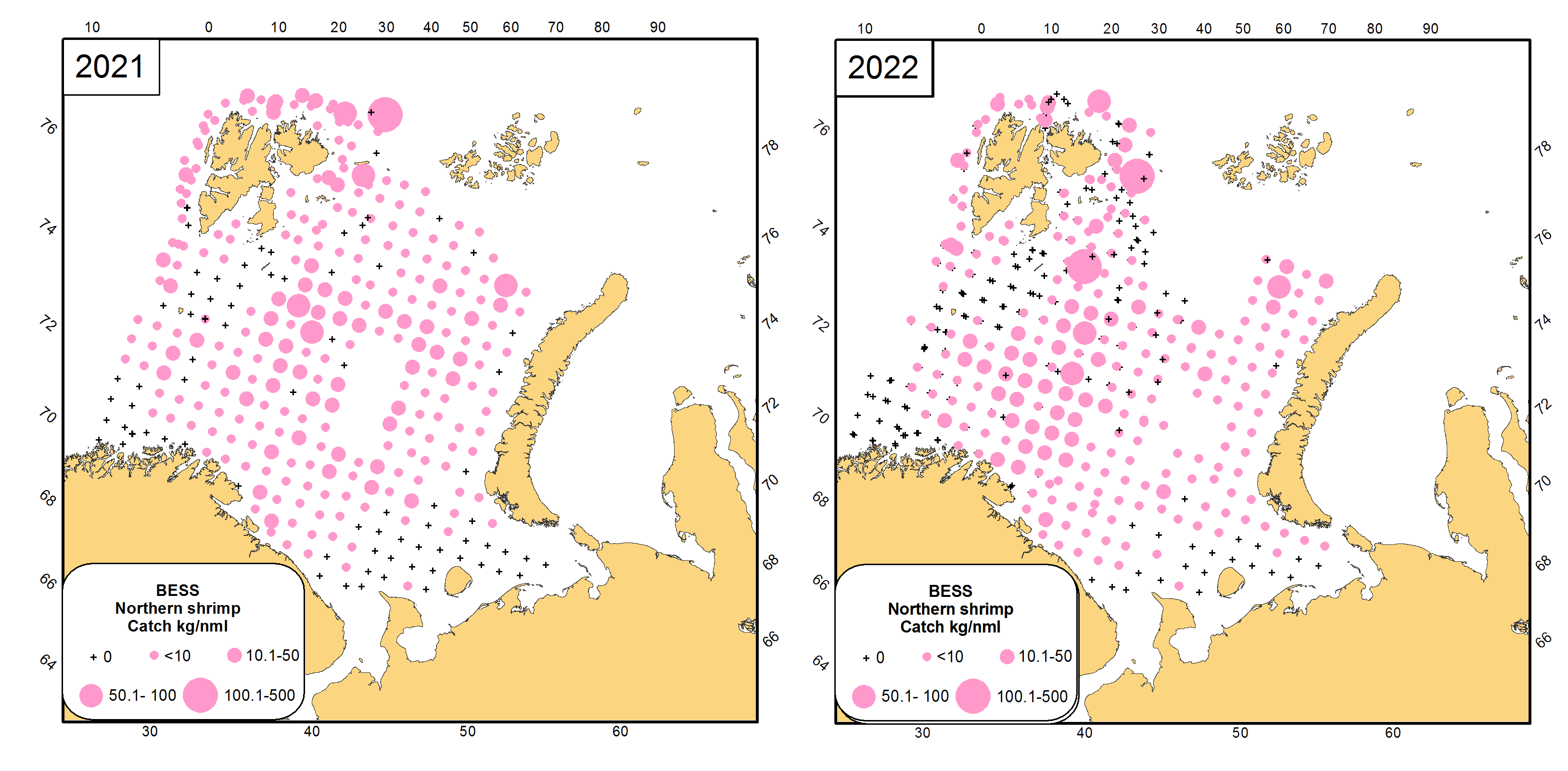
Biological analysis of the northern shrimp was conducted in 2022 by Russian scientists in the eastern part of the survey area. As in 2021, the bulk of the population of the eastern Barents Sea shrimp was made up of smaller individuals, i.e males with a carapace length of 10-25 mm in addition to females with a carapace length of 15-30 mm (Fig. 10.1.2). In 2022 proportion of males and females was almost equal.
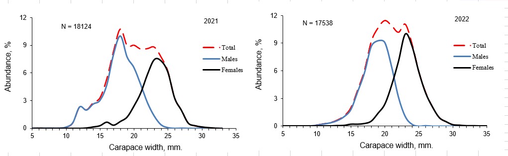
10.2 Red king crab (Paralithodes camtschaticus)
Text by: Aleksei Stesko and Ann Merete Hjelset
Figures by: J. Zhak
During BESS-2022 the red king crab was recorded in 23 of 293 trawl catches: in 1 station in Norwegian water and in 22 stations in Russian part of survey (Table 10.2.1). Compared to previous years, in 2022 there was not recorded any expansion of red king crab range to north or east (Fig. 10.2.1).
Despite the identical coverage of the red king crab area by stations, in 2022 compared to 2021 both the number of recording and the total catch were significantly lower (Table 10.2.1, Fig. 10.2.1).
As in previous years, the most abundant catches were recorded in Russian water near peninsula Kanin Cap.
|
Year |
Total number of station |
Number of station with red king crab |
Total catch, ind. |
Total catch, kg |
|
2005 |
649 |
8 |
106 |
309 |
|
2006 |
550 |
66 |
1243 |
3350 |
|
2007 |
608 |
30 |
1521 |
3869 |
|
2008 |
452 |
10 |
127 |
93 |
|
2009 |
387 |
7 |
15 |
25 |
|
2010 |
331 |
6 |
12 |
25 |
|
2011 |
401 |
4 |
40 |
22 |
|
2012 |
455 |
8 |
126 |
308 |
|
2013 |
493 |
3 |
272 |
437 |
|
2014 |
304 |
11 |
168 |
403 |
|
2015 |
335 |
14 |
255 |
517 |
|
2016 |
317 |
11 |
202 |
552 |
|
2017 |
376 |
13 |
299 |
687 |
|
2018* |
217 |
5 |
73 |
175 |
|
2019 |
323 |
32 |
1635 |
2897 |
|
2020 |
461 |
22 |
233 |
547 |
|
2021 |
341 |
26 |
373 |
1186 |
|
2022 |
293 |
23 |
306 |
1035 |
* reduced coverage of the red king crab area
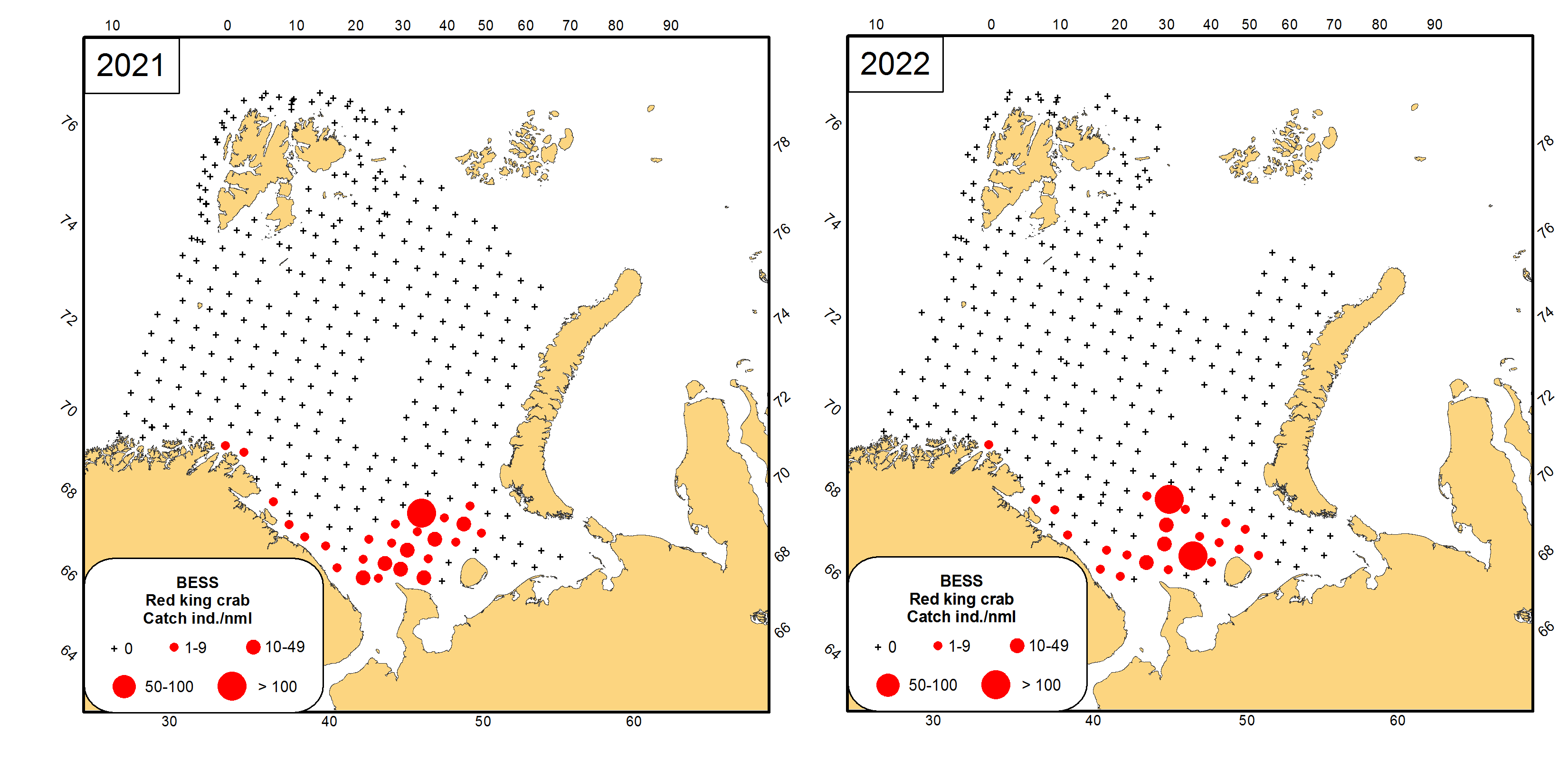
The biomass of red king crab catches in 2022 varied from 4.8 to 548.4 kg/nm compared with 0.8 to 511.6 kg/nm in 2021. The average biomass was 54.3±27.5 kg/nm compared with 54.9±23.8 kg/nm in 2021.
The abundance of crab in 2022 ranged from 1.2 to 149.4 ind./nm given an average crab abundance of 16.1±7.6 ind./nm compared with 1.3-201.2 ind./nm and 17.3±7.7 ind./nm in 2021.
The size structure of the red king crab population in 2022 is characterized by domination of two groups of crabs with carapace width 140-170 and 190-230 mm. (Fig. 10.2.2).
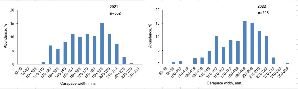
10.3 Snow crab (Chionoecetes opilio)
Text by: Sergei Bakanev, Aleksei Stesko and Ann Merete Hjelset
Figures by: J. Zhak
In 2022, snow crabs were recorded in 95 out of 293 trawl catches. Compared to previous year, the total catch of snow crab decreased, but also the number of stations is fewer compared with previous years. (Table 10.3.1).
During the sampling period, there have been single observations of snow crab outside central Barents Sea. In 2017 the snow crab was for the first-time recorded northwest of Svalbard (Spitsbergen). In 2018 one small male (CW= 34 mm) and weight 12 g was caught south-west of South Cap of Spitsbergen at 350 m. In 2019 and 2020 snow crab was not recorded in the water around Svalbard (Spitsbergen), however in 2021-2022 it was caught in South and the South-eastern part of Svalbard (Spitsbergen) area, but no more than 9 ind./nm.
Within the survey area and stations with catches of crab, the biomass per station in 2022 varied from 0.001 to 6.63 kg/nm with an average 0.671±0.1 kg/nm compared with 0.001 to 18.3 kg/nm with an average 1.3±0.1 kg/nm in 2021 (Fig. 10.3.1, Table 10.3.1).
The abundance in 2022 ranged from 1 to 382 ind./nm with an average of 12.04±3.91 ind./nm compared with 1-398 ind./nm and 19.8±0.9 ind./nm in 2021 (Fig. 10.3.1, Table 10.3.1).
|
Year |
Total number of stations |
Number of stations with snow crab |
Total catch, ind. |
Total catch, kg |
Mean abundance, ind./nm |
Mean biomass, kg/nm |
|
2005 |
649 |
10 |
14 |
2.5 |
1 |
0.3 |
|
2006 |
550 |
28 |
68 |
11 |
3 |
0.5 |
|
2007 |
608 |
55 |
133 |
18 |
3 |
0.4 |
|
2008 |
452 |
76 |
668 |
69 |
11 |
1.2 |
|
2009 |
387 |
61 |
276 |
36 |
6 |
0.8 |
|
2010 |
331 |
56 |
437 |
22 |
10 |
0.5 |
|
2011 |
401 |
78 |
6219 |
154 |
99 |
2.4 |
|
2012 |
455 |
116 |
37072 |
1169 |
395 |
12.6 |
|
2013 |
493 |
131 |
20357 |
1205 |
210 |
12.7 |
|
2014 |
304 |
78 |
12871 |
658 |
206 |
10.5 |
|
2015 |
335 |
89 |
4245 |
378 |
57 |
5.2 |
|
2016 |
317 |
84 |
2156 |
137 |
26 |
1.9 |
|
2017 |
376 |
159 |
25878 |
1422 |
147 |
10.0 |
|
2018* |
217 |
61 |
19494 |
846 |
393 |
16.7 |
|
2019* |
323 |
87 |
15523 |
608 |
145 |
6.6 |
|
2020 |
461 |
141 |
4403 |
436 |
38 |
3.7 |
|
2021 |
341 |
105 |
1705 |
110 |
20 |
1.3 |
|
2022 |
293 |
95 |
891 |
50 |
12 |
0.7 |
* Some stations in the snow crab area were not surveyed in 2018 and 2019
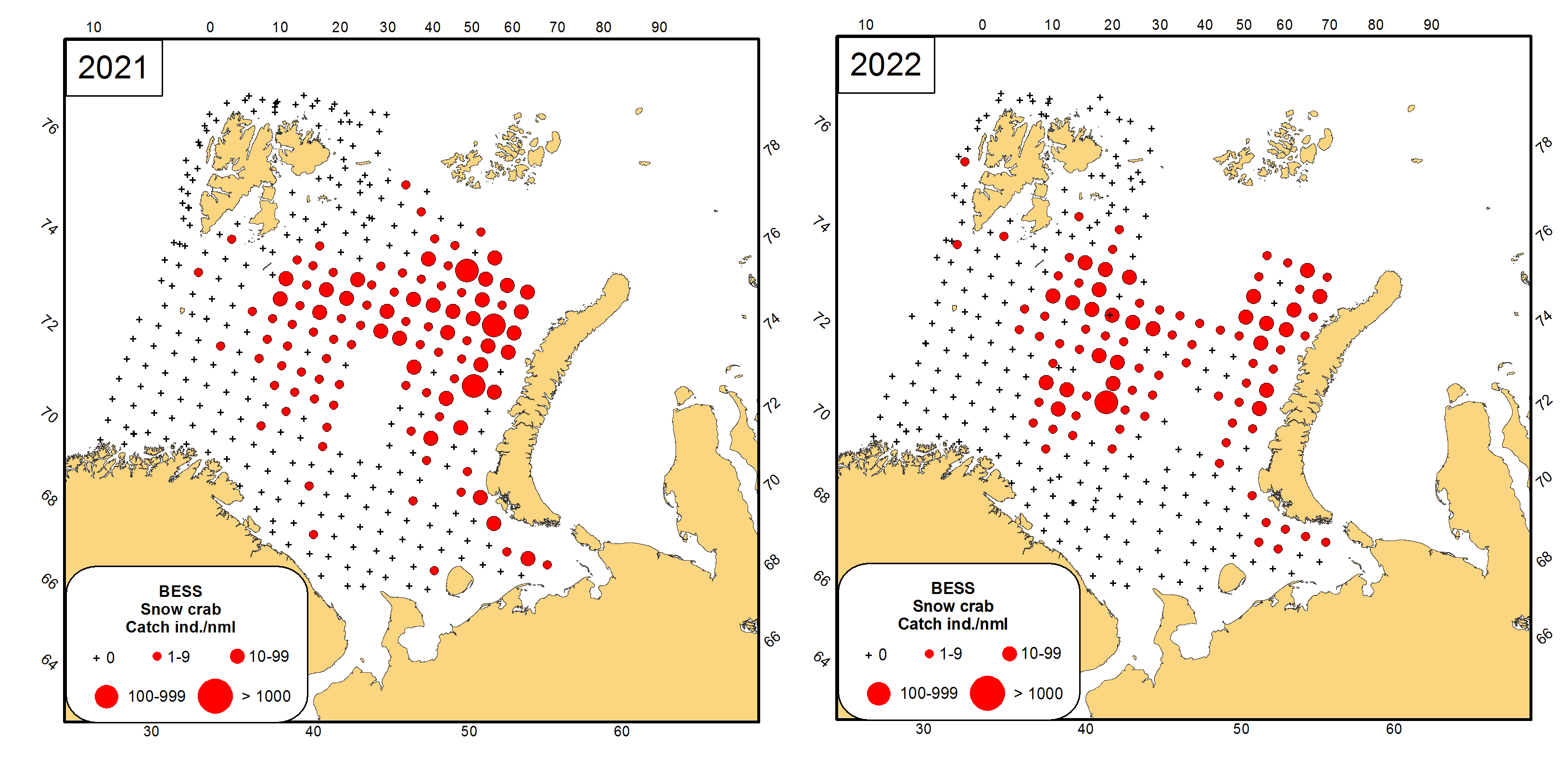
The measured size composition of snow crabs caught in 2022 were dominated by females with 30-40 mm carapace width and males with carapace width 30-40 and 70-100 mm (Fig. 10.3.2 B). The size structure of snow crab catches in 2022 was very close to the structure in 2021 (Fig. 10.3.2).
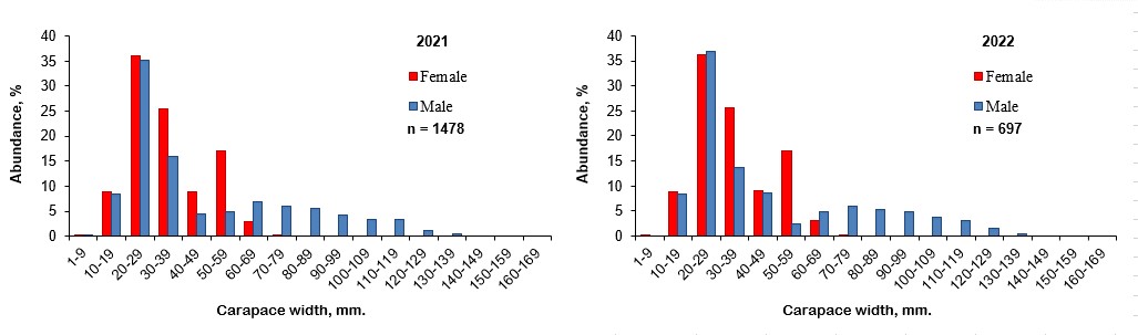
10.4 Iceland scallop ( Chlamys islandica )
Text by: Daria Y. Blinova and Lis Lindal Jørgensen
Figures by: D. Blinova
The Iceland scallop was recorded in 77 of 287 trawl catches in 2022 (Table 10.4.1). The survey showed a wide distribution of scallops in the Barents Sea. The deepest record in 2022 was at 520 m, but the most abundant catches were recorded in the shallow banks and elevations of the bottom is Spitsbergen Bank (Figure 10.4.1).
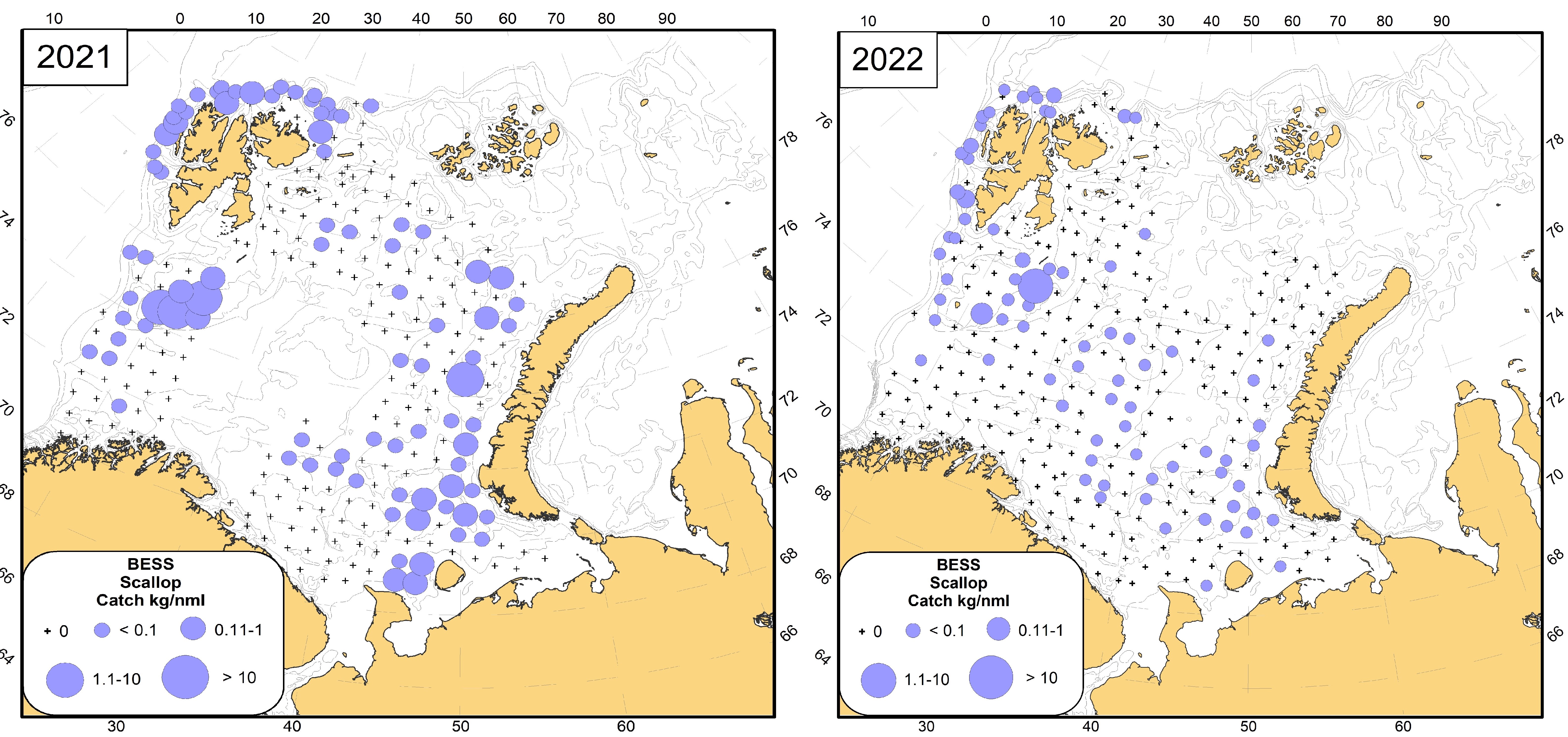
The biomass of scallops in 2022 varied from 0.3 to 2622 g/haul (0.35-2714.75 g/nml). The average biomass is 191.3±37.3 g/haul (224.8±39.9 g/nml) (table 10.4). The abundance ranged from 1 to 276 ind./haul (1-789 ind./nml). The average abundance of scallops is 27±4 ind./haul (34±6 ind./nml).
|
Year |
Stations (% of total) |
Abundance, ind./nml |
Biomass, g/nml |
|
2011 |
101 (26) |
35±5 |
1294±235 |
|
2012 |
146 (33) |
62±7 |
1580±195 |
|
2013 |
131 (27) |
115±17 |
8378±1359 |
|
2014* |
50 (36) |
29±4 |
812±121 |
|
2015 |
103 (31) |
13±1 |
264±32 |
|
2016* |
76 (24) |
18±2 |
268±38 |
|
2017 |
125 (33) |
82±11 |
1486±198 |
|
2018* |
65 (30) |
31±4 |
537±91 |
|
2019* |
112 (35) |
42±11 |
1039±334 |
|
2020 |
97 (23) |
15±5 |
146±40 |
|
2021* |
88 (35) |
20±6 |
225±51 |
|
2022* |
77 (27) |
34±6 |
224.8±39.9 |
* - survey area was not complete
11 - BENTHIC INVERTEBRATE COMMUNITY
Figures by: A. Kudryashova
The list of benthic experts onboard Russian and Norwegian RVs is given in Table 1 (Ch 1).
In 2021, megabenthos was recorded from 254 bottom trawl hauls across four R/Vs during the BESS in 2021. Megabenthos was processed to closest possible taxon with abundance and biomass recorded on all four ships. This was done by two benthic experts from “VNIRO”, and by seven experts from IMR. Benthos was not processed on Part 1 of R/V ”Johan Hjort” due to the absence of benthic experts onboard.
11.1 Species diversity
The total number of megabenthic taxa identified from the trawl-catch across all vessels is presented in Table 11.1. Detailed information about the taxonomic processing onboard the vessels are given in Table 11.2.
A total of 562 invertebrate taxa (382 identified to species level) was recorded in 2022, which is very close to the data of 2021, possible, due to a similar level of the station numbers (Table 11.1). In 2022 68.0 % of benthic invertebrate animals were identified to species level versus 67.1 % in 2021 (Table 11.2).
|
Year |
Number of stations |
Total |
Average abundance, ind./n.ml |
Average biomass, kg/n.ml |
Number |
|||
|
abundance, ind. |
biomass, t |
|||||||
|
species |
taxa |
|||||||
| 2005 |
224 |
83077 |
2.1 |
522.5 |
12.7 |
142 |
218 |
|
|
2006 |
637 |
779454 |
20.7 |
1576.0 |
42.1 |
261 |
388 |
|
|
2007 |
551 |
526263 |
18.2 |
1240.2 |
44.6 |
222 |
351 |
|
|
2008 |
431 |
757334 |
12.2 |
2183.7 |
35.7 |
157 |
244 |
|
|
2009 |
378 |
653918 |
12.3 |
2056.4 |
42.2 |
283 |
391 |
|
|
2010 |
319 |
239282 |
6.8 |
900.0 |
27.3 |
273 |
360 |
|
|
2011 |
391 |
1089586 |
10.8 |
3411.4 |
34.3 |
282 |
442 |
|
|
2012 |
443 |
3521820 |
42.6 |
9832.1 |
125.5 |
354 |
513 |
|
|
2013 |
487 |
1573121 |
27.6 |
3885.0 |
71.7 |
362 |
538 |
|
|
2014 |
165 |
390444 |
5.3 |
2806.7 |
36.7 |
220 |
333 |
|
|
2015 |
334 |
481602 |
5.3 |
1815.1 |
19.9 |
398 |
599 |
|
|
2016 |
317 |
1116405 |
6.8 |
4230.1 |
36.3 |
266 |
423 |
|
|
2017 |
339 |
1073697 |
16.2 |
3769.4 |
58.6 |
319 |
500 |
|
|
2018 |
217 |
852613 |
15.4 |
4887.8 |
89.2 |
404 |
574 |
|
|
2019 |
305 |
1292902 |
19.0 |
4239.0 |
62.5 |
427 |
621 |
|
|
2020 |
429 |
898168 |
10.7 |
1719.1 |
30.4 |
401 |
611 |
|
|
2021 |
254 |
212931 |
10.2 |
1076.6 |
50.6 |
384 |
572 |
|
|
2022 |
283 |
426850 |
5.8 |
2101.2 |
31.3 |
382 |
562 |
|
|
Total: |
6411 |
15 969 467 |
248.0 |
|
|
815 |
1290 |
|
|
Average*: |
370±32 |
795848±100910 |
13.2±1.6 |
2619±319 |
44.6±4.5 |
315±20 |
466±29 |
|
* The average long-term value for the period 2006-2022 except invalid (inflated) abundance and biomass data of 2012.
|
Research vessels |
"G.O. Sars" |
"Johan Hjort" |
"Vilnyus" |
Total |
|
Number of processed hauls |
64 |
93 |
126 |
283 |
|
Phylum |
13 |
13 |
11 |
14 |
|
Class |
28 |
28 |
20 |
29 |
|
Order |
78 |
82 |
58 |
88 |
|
Family |
170 |
179 |
99 |
211 |
|
Species |
248 |
300 |
133 |
382 |
|
Total number of taxa |
368 |
417 |
173 |
562 |
|
Percentage of species identification* |
67.4 |
71.9 |
76.9 |
68.0 |
* calculated as quotient from division of total number of identifications till species to total number of identifications, %.
The taxonomical structure of the Barents Sea megafauna are almost identical between 2021 and 2022 (Fig. 11.1.1), despite the different interannual area coverage (Fig. 11.1.2). Mollusca had the highest number of taxa (124 taxa) followed by Arthropoda (106 taxa), and Echinodermata (89 taxa). Among the mollusks, 56 % of taxa belonged to Gastropoda (70 taxa), 31 % – to Bivalvia (39 taxa), 10 % to Cephalopoda (10 taxa) and the remaining 4 % were distributed between Solenogastres and Polyplacophora. The Arthropoda phylum were primarily presented by Malacostraca (83 taxa) and Pycnogonida (20 taxa); only 3 taxa belong to Hexanauplia and Thecostraca. Among the Echinoderms the most diverse groups was Asteroidea (43 % of taxa), Ophiuroidea (21 % of taxa) and (Holothuroidea (17 % of taxa).
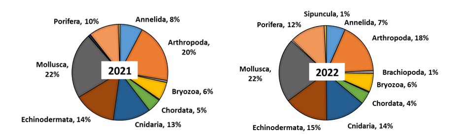
The species density in the terms of the number of taxa in standard trawl catches ranged from 1 to 101 with average of 32.7±1.5 taxa per trawl-catch (versus 29.7±1.4 taxa per trawl-catch in 2021). At the significance level of 0.05, the differences between 2021 and 2022 data are statistically insignificant (p = 0.74).
The lowest level of diversity (1-10 taxa per haul) was recorded in the south-eastern part of the survey area (Fig. 11.1.2). In north-western sector of the sea in the water around Svalbard number of megabenthic taxa reach 101 per station and practically everywhere exceeded 50 taxa per trawling (Fig. 11.1.2)
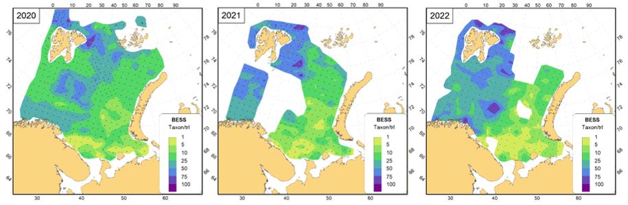
The ten most frequently species taken by trawl in the investigated part of the Barents Sea in 2022 were the decapod crustaceans Sabinea septemcarinata (taken by 67 % of the trawl-hauls), sea stars Ctenodiscus crispatus (65 %), Pontaster tenuispinus (40 %), Henricia species (37 %) and Urasterias lincki (36 %), the brittle stars Ophiopholis aculeate (53 %), Ophiacantha bidentata (47 %), and Ophiura sarsii (40 %), soft coral Gersemia rubiformis (39 %) and polychaetes Spiochaetopterus typicus (37 %).
11.2 New species records
During the BESS 2022, twelve new species was recorded for the first time since 2005 when the ecosystem surveys started (mainly in the Norwegian part of the Barents Sea): decapod shrimp Crangon crangon, bryozoans Carbasea carbasea and Chartella papyracea, sea-squirts Rhizomolgula globularis, sea-stars Luidia sarsii and Culcitopsis borealis, bivalve mollusks Cyrtodaria kurriana and Asperarca nodulosa, gastropods mollusk Propilidium exiguum, and sponges Isodictya palmata, Hexadella dedritifera and Mellonympha mortenseni (Fig. 11.2.1).
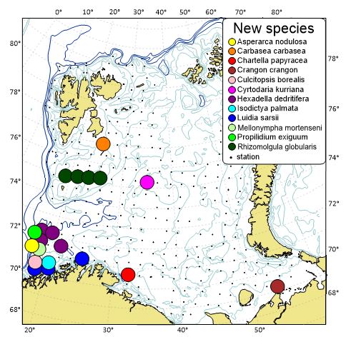
Records of six warm water species (Ch. papyracea, L. sarsii, C. borealis, A. nodulosa, P. exiguum, and M. mortenseni) may be a results of their spreading to the east and north due to the long warming period.
The other new species for the BESS are already known from the Barents Sea and adjacent shelf areas according to literary and Internet sources, and can be a result of a more detailed and/or qualified species identification made by the benthos expert onboard
11.3 Abundance (number of individuals)
The number of megabenthos individuals in the trawl-catches in 2022 (excluding the pelagobenthic species Pandalus borealis) ranged from 1 to 237681 (1-333250 ind./n.ml) with an average of 1590±844 ind. per trawl-catch (2101±1182 ind./n.ml). This is 49 % more than in year 2021 (Table 11.1), what can be caused by interannual variation and difference in station coverage (Fig. 11.3.1).
The largest catch in number of individuals (237681 ind./trawl-catche), mainly consisted of sea-squirt (Ascidiacea) Rhizomolgula globularis (237430 ind./ trawl-catch) was obtained in the western part of the Barents Sea near Bear Island (75.00° N, 19.01° E) at the depth 63 m (Fig. 11.3.1). In 2020 similar extra high abundance of sea-squirts, non identified to species level, (265775 ind./trawl-catch) were recorded in the identical position (75.01° N, 18.95° E) at the depth 61 m. As in previous year, the lowest abundances (less than 50-100 ind. per hall) was recorded in the south-eastern part of the sea within the Russian part of the survey.
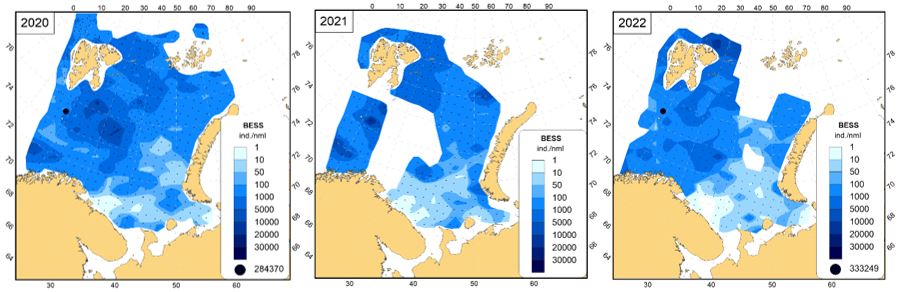
The mentioned extraordinary catch of sea squirts (Chordata in fig 11.2.2) in 2022 changed the distribution of abundance across the main megabenthic groups from the usual dominance of echinoderms and crustaceans to a predominance of ascidians. In 2021 the percentage between the main groups of megabenthos taxa (on the terms of abundance) corresponded to the long-term pattern (Fig. 11.3.2).
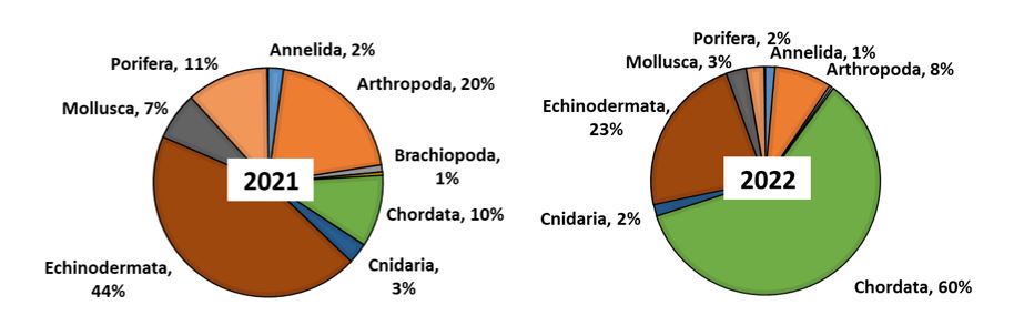
The ten most abundant species (in the term of total number of individuals caught during the BESS 2022) were the sea-squirts Rhizomolgula globularis (66.0 % of total abundance) and Kukenthalia borealis (0.9 %), sea star Ctenodiscus crispatus (5.4 %), shrimp Sabinea septemcarinata (4.1 %), the brittle stars Ophiacantha bidentata (1.8 %), Ophiopholis aculeata (1.3 %), and Ophiura sarsii (1.2 %), sea urchins of genera Strongylocentrotus (in the main S. pallidus) (2.0 %), bivalve Bathyarca glacialis (1.1 %) and barnacle Balanus balanus (0.6 %).
11.4 Biomass
As in previous years, were the main part of the total biomass made up by Sponges, Echinoderms, and Crustaceans (total 94 %), but compared to 2021 had Chordata a slight increase in biomass due to the extraordinary large catch in the Bear Island Bank (Fig. 11.4.1).
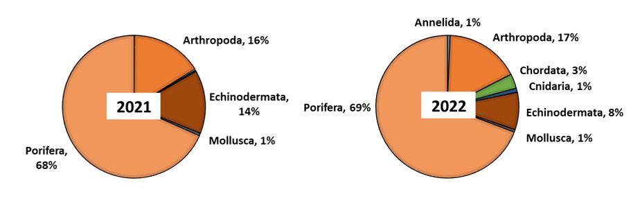
The megabenthos biomass taken by the trawl (excluding the semipelagic species Pandalus borealis) in 2022 varied from 0.003 to 1632 kg (0.004-2197 kg/n.ml) with an average of 21.1±6.7 kg per trawl-catch (31.3±9.7 kg/n.ml). This average is 38.1 % less than in the previous year and 31 % less than the average long-term value for the period 2006-2021 except the invalid 2012 (Table 11.1). The biomass distribution in 2022 was very close to the pattern of previous years (Fig. 11.4.2).
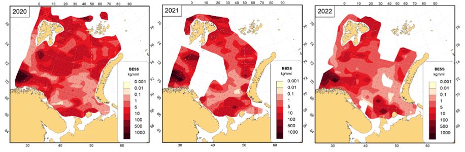
A trawl catch with biomass larger than 1-t was taken in 2022 at one station in the south-western part of the Barents Sea, from 331 m depth (Fig. 11.4.2). This haul was dominated by sponges: Geodia macandrewii (999 kg and 61.2 % of the total station biomass), G. barretti (422 kg; 26.5 %), Stelletta rhaphidiophora (88 kg; 5.4 %), Stryphnus ponderosus (30,5 kg: 1.9 %), and G. phlegrae (29,7 kg; 1.8 %). Other hot spots of biomass (more than 100 kg per trawling) was recorded in Spitsbergen Bank at the depth 93 m (dominated by 197 kg of sea-squirts Rhizomolgula globularis accounting for up to 93 % of the total biomass in the station), north of Spitsbergen (Geodia macandrewii, 90 kg; 82 %), and in the south-eastern part of the sea, north of Kanin Nos peninsula (298 kg of Paralithodes camtschaticus making up to 99,9 % of the total biomass on the station).
More than half of the megabenthic biomass (51.7 % of the total biomass of by-catches) belonged to the Geodia barretti, and G. macandrewii sponges. Other top-dominant species in biomass was crabs Paralithodes camtschaticus (17.3 % of the total biomass), sea-squirts Rhizomolgula globularis (3.3 %), sponges Stelletta rhaphidiophora (2.5 %) and Stryphnus ponderosus (1.6 %), sea stars Ctenodiscus crispatus (2.1 %), and sea-cucumber Cucumaria frondosa (1.3 %). The contribution of each of the other species did not exceed 1% of the total biomass of megabenthos bycatches.
12 - MARINE MAMMALS AND SEABIRDS
12.1 Marine mammals
Due to lack of synchronisation between the Norwegian and Russian part of the 2022 survey, the observatiosn of sea mammals are this time presented in two suchapters, one for each sector.
12.1.1 Marine mammals observed in Norwegian sector
Text by: Nils Øien, Frederike Böhm
Figures by : F. Böhm
During BESS 2022, marine mammal observers were onboard the two vessels Johan Hjort and G.O.Sars which covered the Norwegian sector.
In total, 549 observations were made of groups of marine mammals, comprising altogether a minimum of 2040 individuals. There were eleven marine mammal species identified, of which eight cetacean species and three seal species. Some of the observations were not identified to species but recognized unspecified as either a large whale, dolphin, or seal. The recorded observations are listed in Table 12.x.1 and the distribution of observations by species are given in Figures 12.1.1 (toothed whales) and 12.x.2 (baleen whales).
The dominant species during the ecosystem surveys are the baleen whales minke (Balaenoptera acutorostrata), fin (Balaenoptera physalus) and humpback whales (Megaptera novaeangliae) (Fig. 12.1.1, left). The most constrained distribution of these species is shown by humpback whales which during BESS 2022 were only observed east off Svalbard in the Hopen area and the Olga Strait where they overlap with the traditional capelin concentrations. However, both minke and fin whales are also abundant in this area. In addition, the two latter species have a wide distribution within the surveyed area. The fin whales are especially concentrated in the coastal areas off northern Norway and southwest of Spitsbergen while the minke whales appeared to be associated with the continental slopes from northern Norway to north of Spitsbergen. One blue whale was observed north of Spitsbergen.
| Species | Number of observations | Number of individuals | Group size |
| Unidentified large whale | 12 | 24 | 2,00 |
| Minke whale | 143 | 152 | 1,06 |
| Fin whale | 105 | 314 | 2,99 |
| Blue whale | 1 | 1 | 1,00 |
| Humpback whale | 58 | 87 | 1,50 |
| Unidentified dolphin | 1 | 1 | 1,00 |
| Harbour porpoise | 7 | 11 | 1,57 |
| Killer whale | 1 | 2 | 2,00 |
| White-beaked dolphin | 217 | 1447 | 6,67 |
| Sperm whale | 4 | 4 | 1,00 |
| Unidentified seal | 2 | 2 | 1,00 |
| Harp seal | 1 | 1 | 1,00 |
| Ringed seal | 2 | 2 | 1,00 |
| Walrus | 6 | 15 | 2,50 |
| Totals | 549 | 2040 |
The occurrence of toothed whales was completely dominated by the presence of the white-beaked dolphin (Fig. 12.1.1, right). It is a very common species in the Barents Sea and has extended its distribution northwards in recent years to comprise the shelf areas of Spitsbergen and the Barents Sea north to about 78° to the east of Edgeøya. Other toothed whales observed, however in small numbers, were harbour porpoise (Phocoena phocoena), killer whale (Orcinus orca, 1 individual), and sperm whale (Physeter macrocephalus).
Only a few pinnipeds were observed: Harp seal (Pagophilus groenlandicus), ringed seal (Phoca hispida) and walrus (Odobenus rosmarus). The lack of seal observations during the ecosystem survey is most probably caused by ice free areas. During a whale survey in summer 2022 covering the same areas, many harp seals were registered especially in the areas of Hinlopen and the Olga Strait.
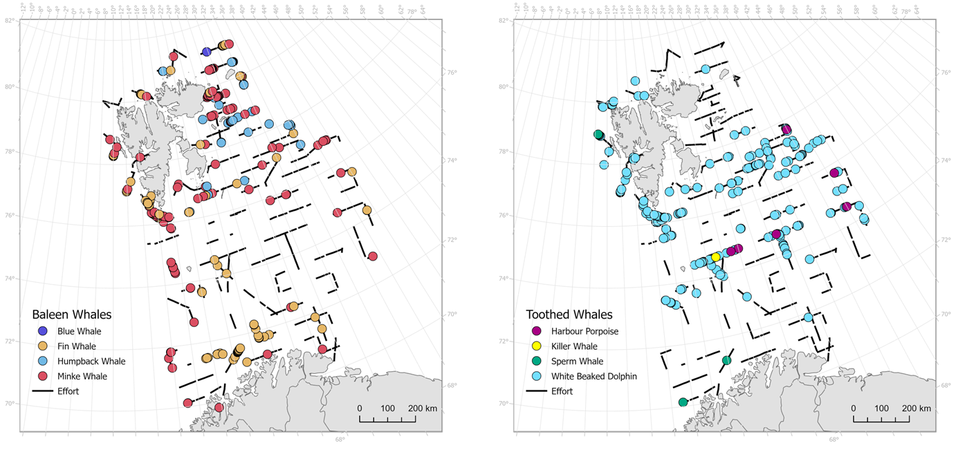
12.1.2 Marine mammals observed in Russian sector
Text and figures by : R. Klepikovskiy
Observations of marine mammals from Russian vessel Vilnyus in the eastern Barents Sea in to 2022 were carried out in end September, end October, November and even first day of December. Due to this, the occurrence of marine mammals was significantly lower compared to observations made at standard times in August-September.
During the observations period, 4 species of marine mammals were registered, with a total number of 195 individuals. Data of observations are presented in the table 12.1.2 and in the figure 12.1.2. The most numerous species was the white-beaked dolphin who was recorded in groups of 2 to 50 individuals, mainly in areas located north of 74º N in places of concentrations of capelin and polar cod. In addition to the white-beaked dolphin, among the toothed whales, only the harbor porpoise was observed, a group of 10 individuals of which was recorded in mid-November in the Pechora Sea on herring concentrations.
Minke whale and humpback whale have been observed among baleen whales. During the research, only 3 observations with minke whale were registered. In December, one humpback whale was recorded near the Murmansk coast.
Such common species as fin whale and killer whale were not observed.
Also this year, due to surveying in more southerly areas far from the ice, pinnipeds and polar bears (Ursus maritimus) were not observed.
| Species | Number of observations | Number of individuals | Group size |
| Minke whale | 3 | 3 | 1 |
| Humpback whale | 1 | 1 | 1 |
| White-beaked dolphin | 25 | 181 | 7,2 |
| Harbour porpoise | 1 | 10 | 10 |
| Totals | 30 | 195 |
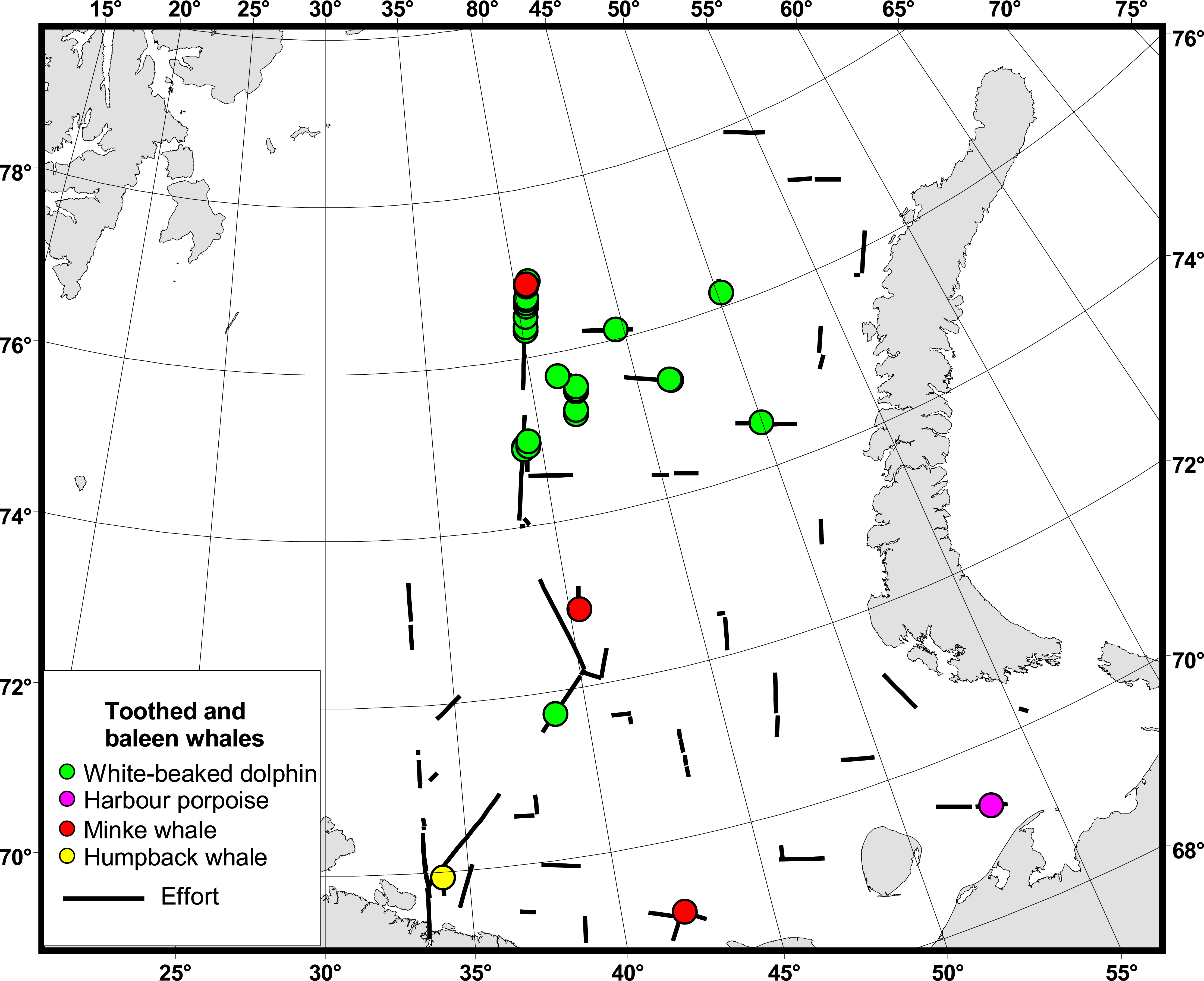
12.2 Seabird observations
Text and figures by: Per Fauchald
Seabird observations were carried out by standardized strip transect methodology. Birds were counted from the vessel’s bridge while the ship was steaming at a constant speed of ca. 10 knots. All birds seen within an arc of 300 m from directly ahead to 90° to one side of the ship were counted. Counts were done only during daylight and when visibility allowed a complete overview of the transect. On GO Sars and Johan Hjort, birds following the ship i.e. “ship-followers”, were counted as point observations within the sector every ten minutes. Ship-followers included the most common gull species and Northern fulmar. On Vilnus, ship-followers were counted continuously along the transects, and by a point observation at the start of each transect. The ship-followers are attracted to the ship from surrounding areas and individual birds are likely to be counted several times. The numbers of ship-followers are therefore probably grossly over-estimated.
The Norwegian sector were covered by GO Sars and Johan Hjort in the period 16 August to 4 October. The Russian sector was covered by Vilnus in the period from 21 September to 1 December. Total transect length covered by GO Sars and Johan Hjort was 7246 km. Total transect length covered by Vilnus was 2959 km. A total of 35 624 birds belonging to 34 different species were counted. The distribution of the dominant auk species is shown in Fig 1 and the distribution of the most common gull species and Northern fulmar is shown in Fig 2. Because several seabird species migrate in and out of the Barents Sea during autumn, the time difference between the coverage of the Norwegian and Russian sectors might cause some biases in the distribution pattern shown in Figs 1 and 2.
Broadly, the distribution of the different species (Figures 12.2.1 and 12.2.2) was similar to the distribution in previous years. For the auks (Figur 12.2.1), high density of little auks (Alle alle) was found north of Spitsbergen. Thick-billed murres (Uria lomvia) were found in the northern part of the Barents Sea with the highest densities east of Spitsbergen. Atlantic puffins (Fratercula arctica) were found in the southern and western Barents Sea and common guillemots (Uria aalge) were found in the southern part of the area. Northern fulmar (Fulmarus glacialis) and black-legged kittiwake (Rissa tridactyla) were encountered throughout the Barents Sea but with highest density in northeast (Figures 12.2.2). For the large gull species, herring gull (Larus argentatus) and great black-backed gull (Larus marinus) were found along the coast of Kola and Finnmark, while glaucous gull (Larus hyperboreus) was mainly encountered in the southeastern Barents Sea and Pechora Sea but was also present in the central and northern part of the area.