Numerical models and long term monitoring

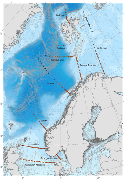
Institute of Marine Research (IMR) conducts 10 fixed transects on a multiannual basis during which hydrographical, chemical and plankton data are collected at the same positions several times a year. Three transects are conducted in the North Sea, four in the Norwegian Sea and three in the Barents Sea and the Arctic Ocean (Figure 1). A 2011 review of the fixed transects (Iversen et al., 2011) records when each of the transects were first occupied, the frequency of occupation and the variables collected along each transect up until 2011. This report also describes specific research questions with which each of the transects were concerned. Due to modifications in sampling and research questions since 2011, an updated description is underway. The transect data sets, which span four or five decades (seven decades in the case of Torungen-Hirtshals and Vardø-North), have been vital to the understanding of long-term variability and trends in environmental and climate conditions, both in Norwegian waters and the wider region. These data are reported to many different national and international agencies including ICES, NFD, the Directorate of Fisheries, the Norwegian Environment Agency, the Norwegian Species Data Bank, State of the Environment, OSPAR and PAEC.

Due to significant pressure on vessel resources, IMR has established a New Monitoring methodology (NEMO) project, as part of which the Oceanography and Climate and the Plankton Research Groups have been asked to consider whether shipboard monitoring may be reduced in favour of new technologies, particularly remotely operated platforms. The fixed transects place a considerable demand on ship time, amounting to on average 43 transects during a year (20 in the North Sea, 14 in the Norwegian Sea and 9 in the Barents Sea-Arctic Sea). This report examines how hydrographic data generated by numerical models developed and/or intensively used by scientists in the Oceanography and Climate Research Group can be utilised to assess and support the shipboard monitoring. The following objectives have then been defined:

1. Assess how well existing model products reproduce variability and trends in regional hydrography and/or ocean currents over interannual to multidecadal timescales.

2. Apply numerical models to assess how well the present sampling strategy captures the spatial variability in hydrographic variables and outline how the model can be used to determine the sampling frequency.

3. Determine the extent (or for which purposes) numerical products may be used as a support for in-situ data.

2.1 - Numerical model data

Several global (low resolution) and regional (higher-resolution, eddy resolving) ocean models have been developed which describe hydrographic conditions in Norwegian waters and the surrounding region. Data from three such models (TOPAZ, Norkyst and NEMO-NAA10 km) are used in this report. These model products have been chosen as they have each been developed with the support of scientists in the Oceanography and Climate Group. TOPAZ and NEMO-NAA10 km are both regional ocean models, coupled to a sea ice model, and nested within a global earth system model. The latest version of Norkyst applied in this report is nested within TOPAZ and then covers a much smaller domain. The models differ considerably from each other, each using a different model framework and grid and different lateral and atmospheric forcings. It is important to consider that each model has been developed with a different intended application in mind. The three models have been described in detail in previous publications and reports (see references below) and as such only a very brief description of each is provided here.

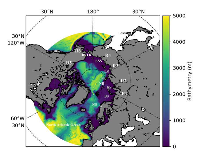
TOPAZ: The TOPAZ Arctic Ocean Physics Reanalysis is provided by the Copernicus Marine Service and can be accessed via https://doi.org/10.48670/moi-00007. It uses a recent version of the Hybrid Coordinate Ocean Model (HYCOM) developed at the University of Miami (Bleck 2002), coupled to a sea ice model. The model's native grid which covers the Arctic and North Atlantic Oceans (Figure A1, Appendix 1), has fairly homogeneous horizontal spacing (between 11 km and 16 km) and 50 hybrid layers. TOPAZ is a product generated from the mean of a 100-member model ensemble (where the ensemble aims to span a range of possible model parameterizations, thus reducing parameterisation errors). The data are interpolated onto a standard grid with 12.5 km x 12.5 km horizontal resolution. TOPAZ is the only model system considered here to assimilate observations, with data assimilation performed on a weekly basis. It should be noted that IMR cruise data are included in the assimilation system. If the goal was to assess if TOPAZ can replace in situ sampling, the version of TOPAZ without data assimilation should be consulted instead. However, our goal is to assess how the model can be used to support the in situ sampling and to assess sampling strategy. Earlier studies have shown that adding observations into TOPAZ in general increase the skill in reproducing the observations (Lien et al., 2016). Moreover, data that are rather sparse in time and space will have a limited effect on the increments used in the data assimilation. Based on this, we concluded that the version with data assimilation is most suitable for this evaluation. TOPAZ is run operationally, and for this study we used daily mean model hindcast data for the period 1 Jan 1991 to 31 Dec 2022.  Biogeochemical and lower trophic level variables generated by ECOSMO coupled to HYCOM (Yumruktepe et al., 2022) are also available via the Copernicus web portal and are interpolated onto the same grid as the physics data.

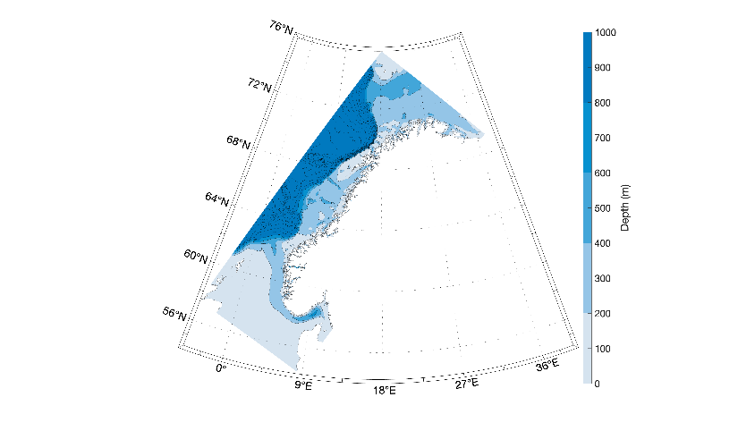
Norkyst: The Norkyst model system applies the ROMS (Regional Ocean Modelling System (http://www.myroms.org); Shchepetkin and McWilliams, 2005 and Haidvogel et al., 2008) to the Norwegian coastal zone (Figure A2, Appendix 1). The model has a horizontal resolution of around 800 m x 800 m and has been demonstrated to represent the physical environment in the sea areas around the Norwegian coast including in the largest fjords. More details are provided in  Albretsen et al. (2011), (2012) and Asplin et al. (2020). A historic hindcast is currently available spanning the period 2012 to today and MET-Norway generates 5-day forecasts every day using the exact same model system2023. Norkyst uses data from the TOPAZ model products as open boundary conditions and can thus be considered a downstream coastal application of the Copernicus Marine Service products.

NEMO-NAA10 km: NEMO-NAA10 km (NAA stands for North Atlantic & Arctic) is a new regional model configuration based on the NEMO version 3.6 (Madec & the NEMO system team, 2015), recently developed at IMR (Hordoir et al., 2022). The model spans the North Atlantic and Arctic Ocean (Figure A3, Appendix 1) with a horizontal resolution of 10 km on average. A historic hindcast is currently available spanning the period 1998 to 2023.

A version of NEMO covering the North Sea and Northwest Shelf is run operationally as part of the Copernicus Marine Service (like TOPAZ for the Arctic region). This model product is not utilized here but could be considered for studies focusing on the North Sea region.

The three models described above have been previously demonstrated to recreate hydrographic conditions in Norwegian waters and the surrounding seas with significant skill (e.g. for TOPAZ; Lien et al. (2016) and Yumruktepe et al. (2022), for Norkyst; Albretsen et al. (2011) and Asplin et al. (2020), and for NEMO-NAA10 km; Hordoir et al. (2022)). However, TOPAZ is the only fully operational model with a model domain covering all the transects considered here. Thus, in the following assessment of model skill, we focus on interpreting how well TOPAZ reproduce trends and variability over multi-annual to multi-decadal timescales. Thereafter, we compare modelled velocities from all the three models to current measurements. As current measurements are not assimilated into TOPAZ, that assessment is conducted towards an independent data set for all three models.

2.2 - In-situ data

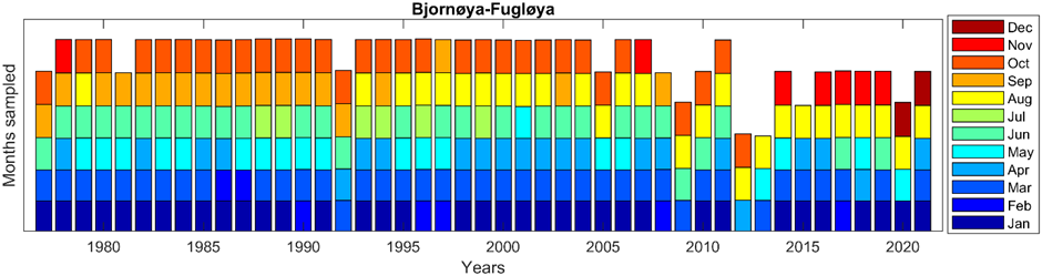
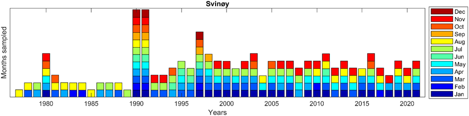
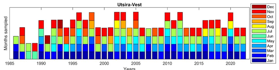
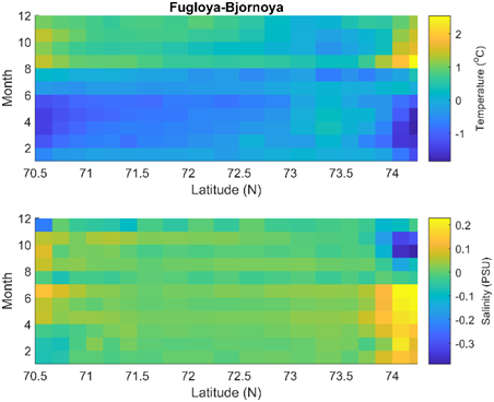
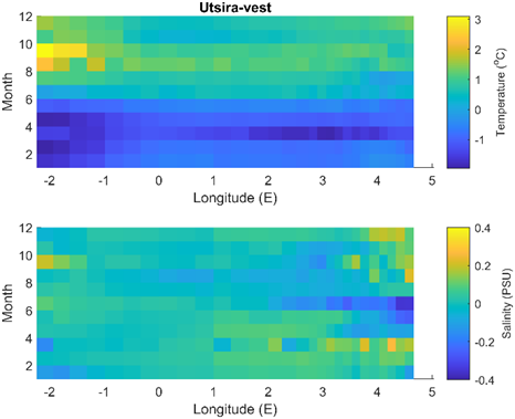
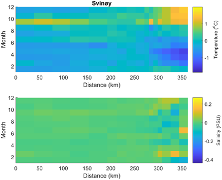
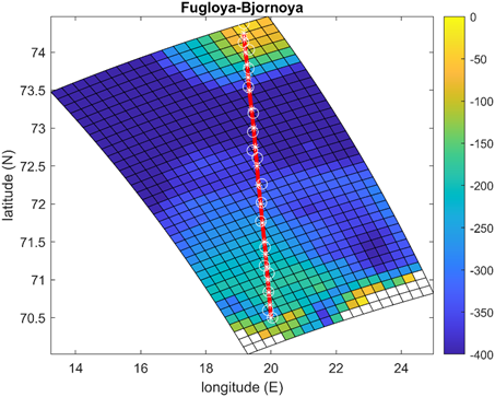
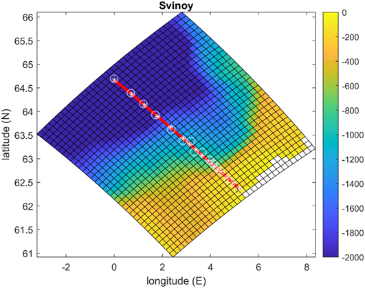
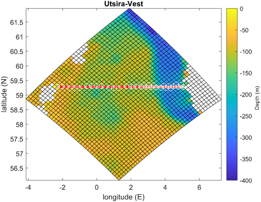
CTD data: Temperature and Salinity data (1991-2021) from three of the fixed transects conducted by IMR are used in this study, these being Utsira-West in the North Sea, Svinøy in the Norwegian Sea, and Bjørnøya-Fugløya in the Barents Sea. The number of samples collected per year and the seasonal spread of the data have varied over time as indicated by the Figures in Appendix 2 (Figures A4-A6). Typically, the transects were occupied less frequently during the early years of data collection. As the CTD data are not distributed uniformly throughout the year, it was necessary to remove the seasonal signal from the data before calculating the annual means used to derive long term trends. The seasonal cycles vary considerably along the length of each transect meaning this must be done on a station-by-station basis, particularly when comparing coastal and offshore regions (see Figures A7-A9 in Appendix 3, which show the depth mean seasonal cycle for each station along each of the transects).

While several approaches were tested for deseasonalising the data, a simple approach proved most effective: The mean seasonal signal at each individual station was calculated, averaging all available data from the record over monthly intervals. The estimated monthly mean seasonal anomaly was then subtracted from each data point prior to calculating annual means. The seasonal cycle cannot be removed precisely and constitutes the largest source of error in the estimation of annual mean temperature and salinity values from the CTD data. We note here that the time series estimation for Fugløya-Bjørnøya and Svinøy transects are conducted over a region which have been chosen to represent key water mass characteristics (see e.g., Figs. 2 and 3). This means that the variation of the seasonal cycle along the transect is of little importance. It also means that the seasonal cycle in the near surface waters, which clearly is the dominant part of the seasonality, is not relevant.

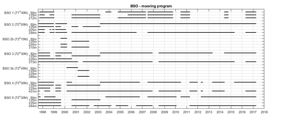
Current data: To assess model skill in representing observed velocities, we make use of a mooring array deployed by IMR across the Barents Sea opening to monitor the inflow of Atlantic Water into the Barents Sea. 26 years of temperature and velocity data have been collected, extending from 1998 to 2023. The number of moorings deployed, and their functioning varied over time, but the general setup was five moorings deployed between 71.5 N and 73.5 N, with a distance of about 55 km between moorings (BSO1 at 71.5 N, BSO2 at 72.0 N, BSO3 at 72.5 N, BSO4 at 73 N and BSO5 at 73.5 N). From August 1999 to March 2002 two additional moorings were included in the mooring array to increase the horizontal resolution to about 25 km (BSO2b at 72.25 N and BSO3b at 72.25 N). See Table 2, Appendix 3 for further details on the temporal distribution of the data at each station over the period 1997-2018. Further details can be found in Ingvaldsen et al. (2004) and the data are freely available from the NMDC (Ingvaldsen, 2020). The instrumentation on the moorings was mostly Aanderaa RCM7 and RCM9 before 2017, and RDI Workhorse/Quartermasters after 2017. From the available data, monthly mean and daily mean time series have been generated.

3.1 - Assessment of TOPAZ skill in reproducing temperature and salinity time series

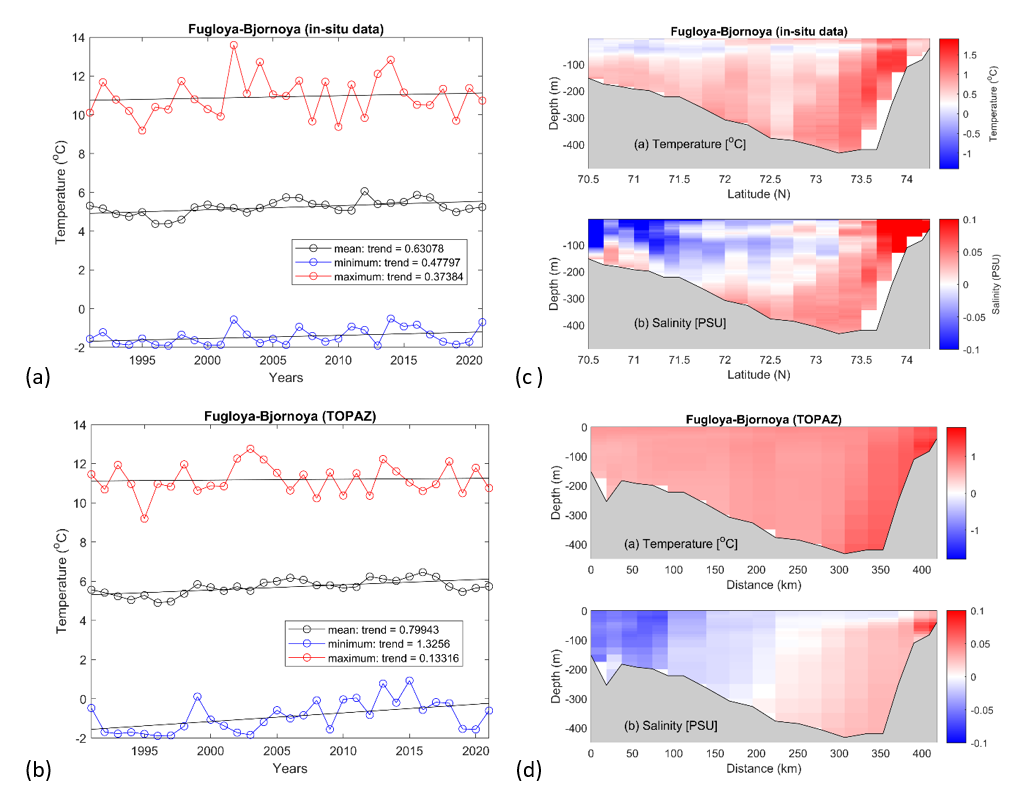
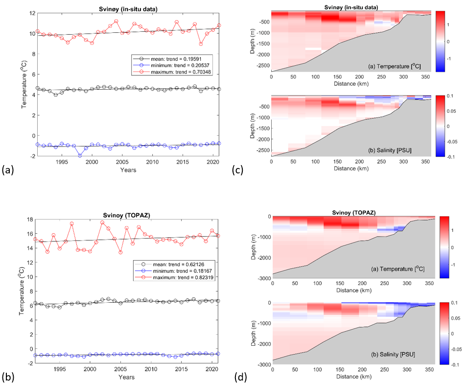
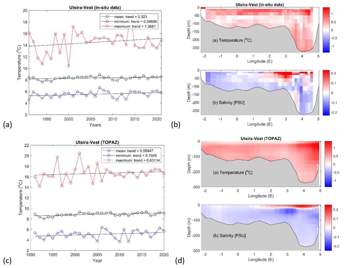
In this section we assess how well time series extracted from the TOPAZ product represent the observed interannual variability and long-term trends in water temperature and salinity along the Utsira-West, Svinøy and Bjørnøya-Fugløya sections. The comparison is conducted over the time period covered by TOPAZ (1991-2021). Temperature and salinity time series from Utsira-West, Svinøy and Bjørnøya-Fugløya are submitted on an annual basis to the ICES Report on Ocean Climate, and derivations of these data can be accessed from the ICES data portal at https://ocean.ices.dk/core/iroc or complete data series from https://www.imr.no/forskning/forskningsdata/operasjonelledata (in Norwegian). The time series are averaged over areas of different sizes as indicated by the boxes in Figures 2a - 4a. These regions have been chosen to represent key characteristics for Atlantic Water. Direct comparisons between the time series generated from the in-situ data, as submitted to ICES, and identical time series generated from TOPAZ are presented in Figures 2b-4b.

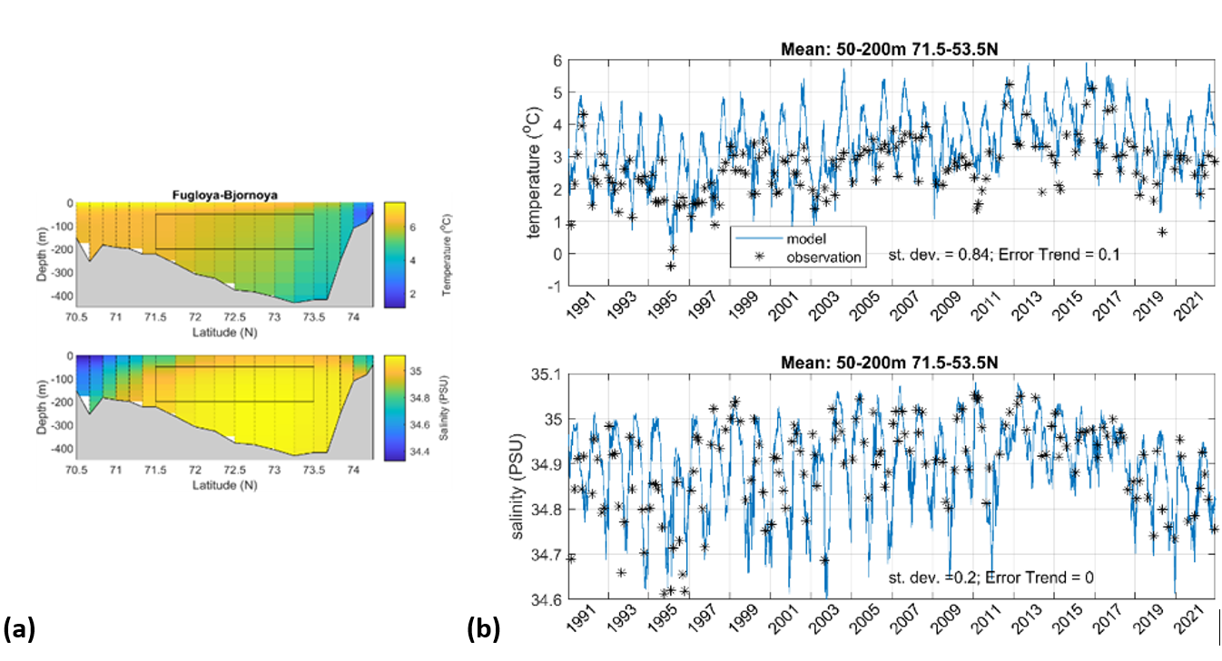
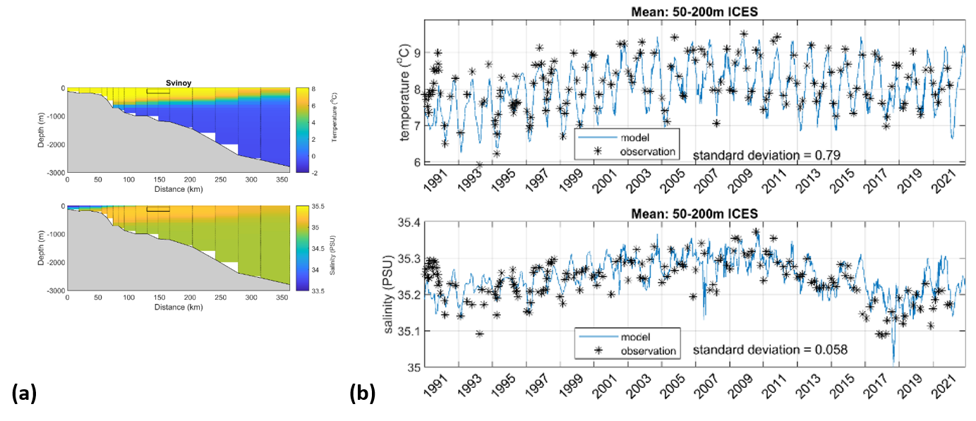
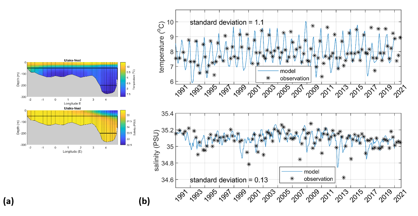
Multiannual variability and long-term tends along the Fugløya-Bjørnøya (Figure 2b), Svinøy (Figure 3b) and Utsira-West (Figure 4b) transects are well represented by TOPAZ, likely due to the assimilation of CTD data. The seasonal amplitude in salinity is also well represented as is the seasonal amplitude in temperature at Svinøy and Utsira-West. It is notable, however, that TOPAZ poorly describes the seasonal amplitude in temperature along the Fugløya-Bjørnøya section, where maximum annual temperatures are overestimated by up to 1.8 ^o C. The reason for this is unclear, considering that the CTD data are assimilated into the model system. However, during the assimilation process, observational data are partially smoothed, while the model itself is continually driven by external forcing, so the model state cannot be equal to the observations even after assimilation. Given that the deviation is mostly in maximum (summer) temperatures, it is possible that the summer heated surface layer in TOPAZ is too deep, thereby including the seasonal signal of the surface layer into the time series. It is also possible that small-scale dynamics that cannot be resolved by the model play a significant role in modulating seasonal temperature cycles in this region.

The TOPAZ system is updated on a biannual basis, and the multidecadal hindcast is not immediately reproduced following each update. Therefore, it is important to consider the possibility of temporally varying biases in the TOPAZ product (for example due to changes in the model formulation, the model grid or the data assimilation scheme). To test this possibility, the trends in temperature and salinity error along the Fugløya-Bjørnøya transect have been calculated. The error trends were found to be insignificant, supporting the suitability of TOPAZ for long-term monitoring studies.

3.2 - Assessment of TOPAZ skill in reproducing observed multi-decadal trends in temperature and salinity

In the following section we assess how well TOPAZ reproduces multi-annual variability and multi-decadal trends in temperature and salinity along the Fugløya-Bjørnøya, Svinøy and Utsira-West transects. It is of interest to determine how well the model represents changes in extremes as well as in mean conditions. For this reason, we compare modelled and observed linear trends in annual mean temperatures averaged across each of the sections over the period 1991-2021 (Figures 5-7a,b) and in the instantaneous minimum and maximum temperatures observed at any location along the transect during each year. The TOPAZ and in-situ time series exhibit similar interannual variability and trends in temperature when averaged across the entire section. At the Svinøy section, however, TOPAZ gives substantial (~4-6^oC) higher maximum temperatures than the observations, and about ~2^o C higher mean temperatures than the observations (Fig. 6a-b). The reason for this is unknown. As previously mentioned, there is considerable variability in hydrographic conditions along the length of the transects. The spatial scales over which the model has skill are also of interest, hence linear trends in temperature and salinity have been calculated at each individual CTD station and depth. The contour plots in Figures 5-7c,d show how temperature and salinity trends vary along the length of each transects.

Each of the transects considered here exhibits a warming trend, although the rate of warming is not consistent along the length of the transect or with depth. Along the Fugløya-Bjørnøya transect, water temperature has warmed nearly twice as fast in the north of the transect as it has in the south. Along the Svinøy transect warming has occurred at a faster rate within the upper approximately 500 m than at depth, while there is evidence of cooling in a small region approximately 8 km offshore and 800 m deep. Along Utsira-West, the warming trend is most significant in the east of the section adjacent to the Norwegian coast. These spatial differences in warming trends reflect the different mechanisms dominant in driving regional warming (i.e. the advective transfer of heat, vertical mixing processes and surface heat exchanges). Further investigation of these patterns is merited to better understand these mechanisms. Here, however, it is important to note that the spatial variability in the warming trends is consistent between TOPAZ and the observations. Thus, any analysis of regional warming trends will benefit from the more complete spatial coverage provided by TOPAZ. (Note that the extent to which model performance can be attributed to data assimilation as opposed to model representation of mechanistic processes is unclear. Data assimilation allows the model to represent the consequences of processes it may not internally resolve.)

Salinity shows regions of both increasing and decreasing trends along each of the transects. Again, there is a high degree of consistency between the spatial patterns of the trends calculated from TOPAZ and from the in-situ data. Along Fugløya-Bjørnøya there is a decreasing trend in salinity in the south of the transect and an increasing trend in the north. Salinity has increased along much of the Svinøy transect except in east of the section on the Norwegian shelf where there has been a freshening trend. By comparison, at Utsira-West, freshening has occurred along most of the transect except in the upper few hundred meters of the eastern half of the transect. The spatial differences in salinity trends reflect the different mechanisms dominant in driving regional change (i.e. advective transfer, vertical mixing processes, surface freshwater exchange and riverine input).

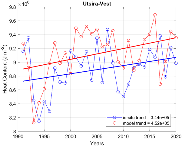
3.3 - A comparison of heat content estimated from in-situ and model data

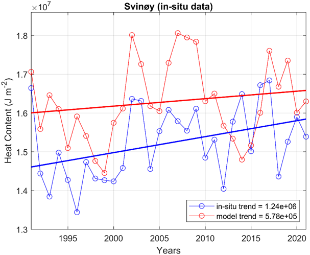
In the previous two sections it has been demonstrated that TOPAZ is able to represent multi-annual variability and multi-decadal trends in temperature and salinity with skill, although clear deviations in absolute values were present for Fugløya-Bjørnøya seasonal maximum temperatures (Fig. 2) and Svinøy annual trends (Fig. 6). Modelled and observed absolute temperature values may differ by more than a degree, which can translate into large errors when estimating heat content (HC), a variable of potential interest to climate change studies. Therefore, we also assess how well TOPAZ reproduces trends in heat content. For this purpose, time series of the annual mean heat content within a 1 m³ column of water have been calculated at stations near the centre of each transect (Figures 8-10). For this we use annual mean depth-time series of temperature and salinity following Equation 1, with the reference temperature (T(z) -Tref) equal to zero;

[Equation 1]

where the heat capacity Cp is calculated as a function of the local temperature T and salinity S, ρ is water density and dz the vertical distance over which the data are averaged. In calculating heat content, annual mean temperature time series were used (annual mean in-situ time series were calculated from the de-seasonalised data).

Fig. 8 shows a comparisons of annual mean heat content at 72.25 N, halfway along the Fugløya-Bjørnøya transect, calculated using TOPAZ and in-situ data. The two time series exhibit similar interannual variability in heat content with a significant shift (increase) in heat content around 2004. The increasing trend in heat content, the absolute values and interannual differences are, however, considerably larger in the model time series than the in-situ time series. This likely reflects the overestimation of the summer maximum temperatures by TOPAZ (Fig. 2). By comparison, absolute values of heat content and long-term trends estimated from in-situ and model data are similar for the Svinøy (Fig. 9) and Utsira-West (Fig. 10) cases. The time series from all three transects indicate moderately warm conditions during 1991, followed by a cool period throughout the rest of the 1990’s, and then warmer conditions after 2000.

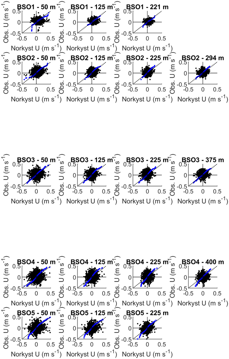
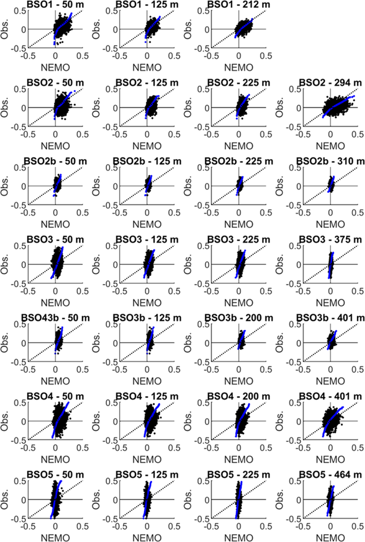
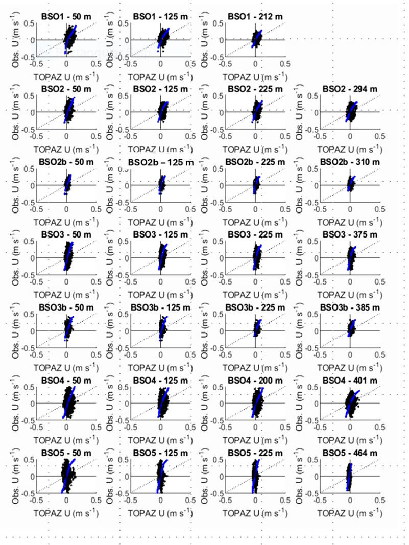
It has been reported previously that TOPAZ underestimates surface drift velocities by 50%, while geostrophic velocities are biased by more than –5 cm s^-1 (Copernicus Marine Services, 2023). For this reason, two additional models are included in the analysis of modelled velocity structures (Norkyst and NEMO-NAA10 km). Current meter data collected across the Barents Sea opening (see section 2.2) have been used to determine how well each of the three models represents observed velocity in this region. We compare 11-years of data extending from 2013-2023 for Norkyst and 25 years of data extending from 1998-2023 for NEMO-NAA10 km and TOPAZ. Velocity time series were extracted from each model at the nearest model grid point to the mooring locations. Model data were then interpolated vertically onto the depths of the current meters and daily mean time series were generated from both the observations and the model data. Scatter plots and quantile-quantile plots (Figs. 11-13) were produced at each location and depth, comparing modelled and observed easterly velocity (velocity into the Barents Sea). Quantile-quantile plots reveal how well the models represent the observed range in current speeds. Considerable differences in model performance are apparent: Norkyst reproduces the observed range of velocities at each location well (Fig. 11), while both NEMO-NAA10 km (Fig. 12), and TOPAZ (Fig. 13) exhibit a negative bias of more than 50%.

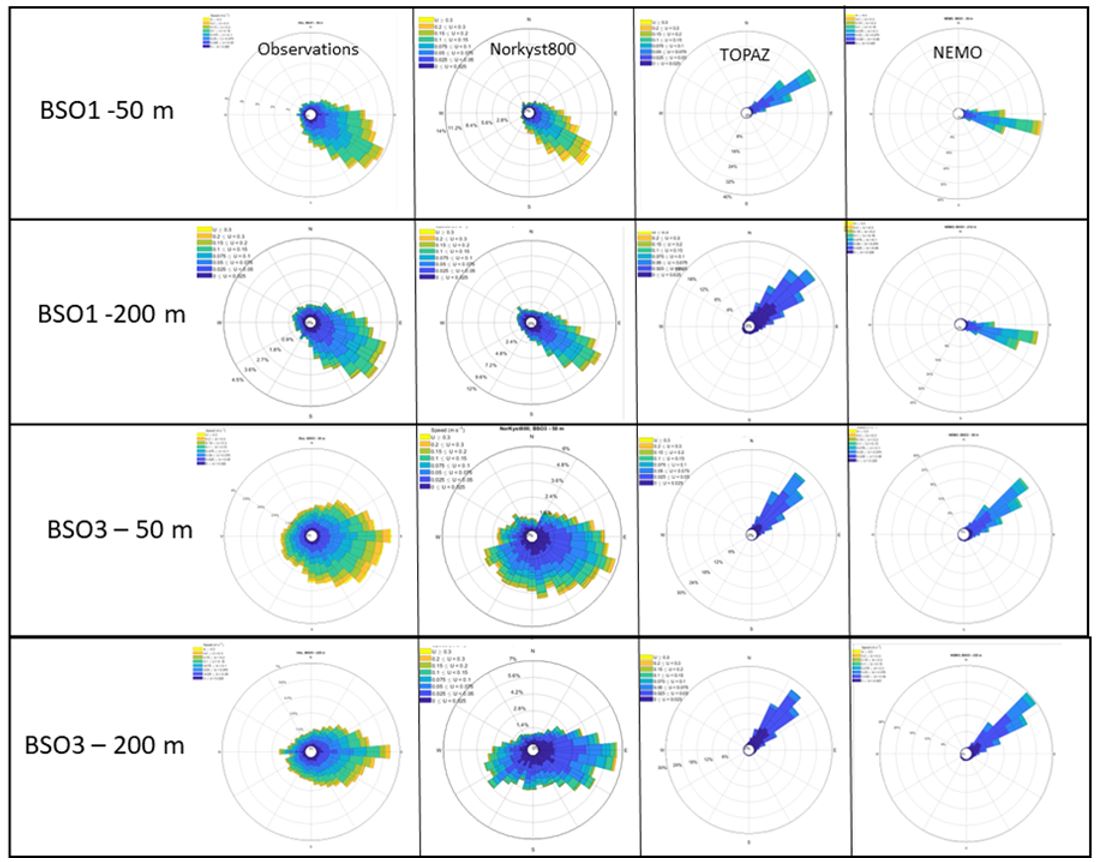
The differences in model performance are exemplified further in current rose diagrams in Fig. 14. Current roses map the frequency of occurrence of currents within a range of defined speed and direction bands, and also illustrate the most prevalent current speed and direction. Current roses are presented for two stations (BSO1 and BSO3) at 50 m and 200 m depth. Norkyst reproduces the observed variability in current speed and direction well at each location and depth, showing the relatively persistent transport into the Barents Sea at BSO1 (the most southerly station) and the more variable transport at BSO3 in the centre of the current meter transect. By comparison, both NEMO-NAA10 km and TOPAZ exhibit limited variability in current direction, with almost no westward transport (i.e. no transport out of the Barents Sea). Mean current directions computed by both NEMO-NAA10 km and TOPAZ are rotated by between 30-40^o to the left of the mean observed flow direction at BSO1 and BSO3.

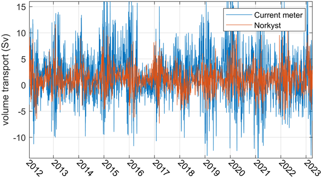
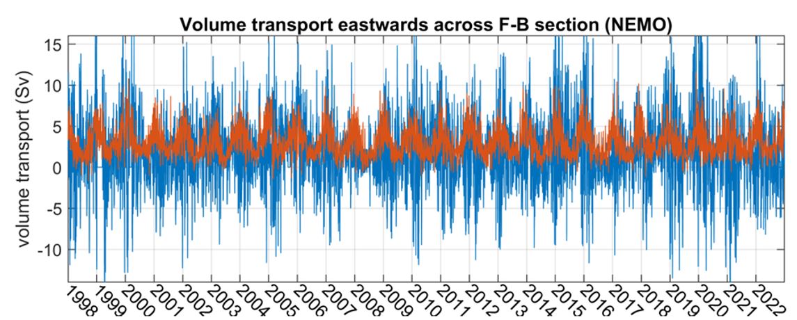
The above methods compare the mean properties of the flow but give no indication of the temporal variability which is of most interest here. For this purpose, total eastward volume transports along the Barents Sea opening section (between BSO1 and BSO5) has been estimated from the observations and from each of the models. While none of the models are able to represent the temporal variability of the eastward transport into the Barents Sea over sub-monthly time scales, both Norkyst (Fig. 15) and NEMO-NAA10 KM (Fig. 16) represent the seasonal variability, characterised by stronger eastward transport during the winter months and weaker flow during the summer months.

5.1 - Impact of sampling frequency on the estimation of annual trends and variability in Atlantic Water flow

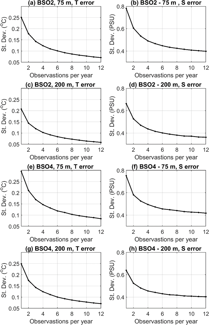
Having demonstrated that TOPAZ recreates multiannual variability in temperature and salinity fields with reasonable skill, despite regional deviations in absolute amplitudes, it is then possible to use TOPAZ to estimate the impact of sampling frequency on long term monitoring of annual trends and variability in the Atlantic Water flow. For this, an approach similar to that described in Rapport fra Havforskningen Nr. 15-2011 (vedlegg 2) has been followed. Daily mean temperature and salinity fields spanning the period 1991-2022 along the Fugløya-Bjørnøya transect were extracted from TOPAZ. Mean seasonal cycles of temperature and salinity were then calculated for each individual station along the transect. The 32-year mean seasonal cycles were smoothed using a 5-day running mean. For a range of sampling frequencies between 1 and 12 per year, the required number of samples was then selected at random from each year of the time series, assuming only one (or zero) sample per month during each year. Annual mean anomalies of temperature and salinity were calculated from the sub-sampled data and compared to the anomalies calculated from the complete (daily) time series. This method was repeated 1000 times for each location and depth of interest and the mean standard deviations between sub-sampled and complete time series are presented in Fig. 17.

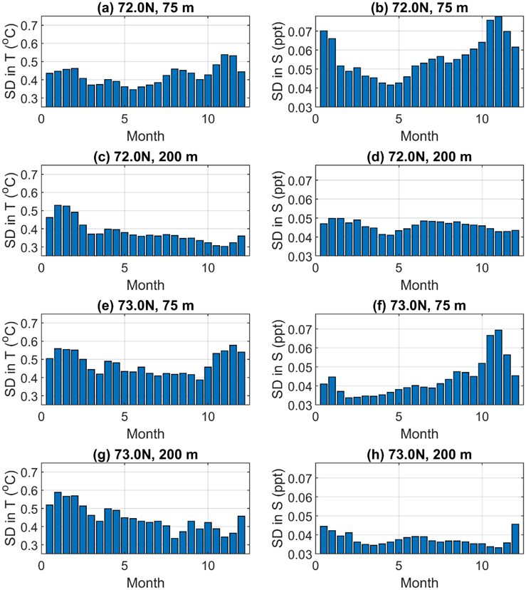
Using the data presented in Fig. 17, it can be determined that increasing the sampling frequency from 1 to 3 observations per year leads to an average reduction of 43% in the standard deviation in temperature error and 29% in the standard deviation of salinity error. Increasing the sampling frequency from 1 to 4 observations per year gives mean reductions of 50% and 34% and from 1 to 5 observations per year gives mean reductions of 56 % and 37 % in the standard deviation of temperature and salinity errors respectively. Thus, it can be argued that there is significant gain in occupying the Fugløya-Bjornøya transect 3 to 4 per year, while increasing the sampling frequency further gives little gain on the annual mean. The months which are best to sample maybe those with the smallest standard deviation over interannual timescales. However, this is dependent on location and depth and differs for temperature and salinity (e.g. Fig. 18). Along the Fugløya-Bjørnøya section, the standard deviation in salinity is on average smallest during March, while the standard deviation in temperature is on average smallest during October, although also relatively low during March meaning springtime may be an optimum time to sample. It is possible to utilise the model to estimate which months are the best to sample, depending on the number of times a transect will be occupied per year.

5.2 - Using model data to determine correlation length scales for the Atlantic Water flow

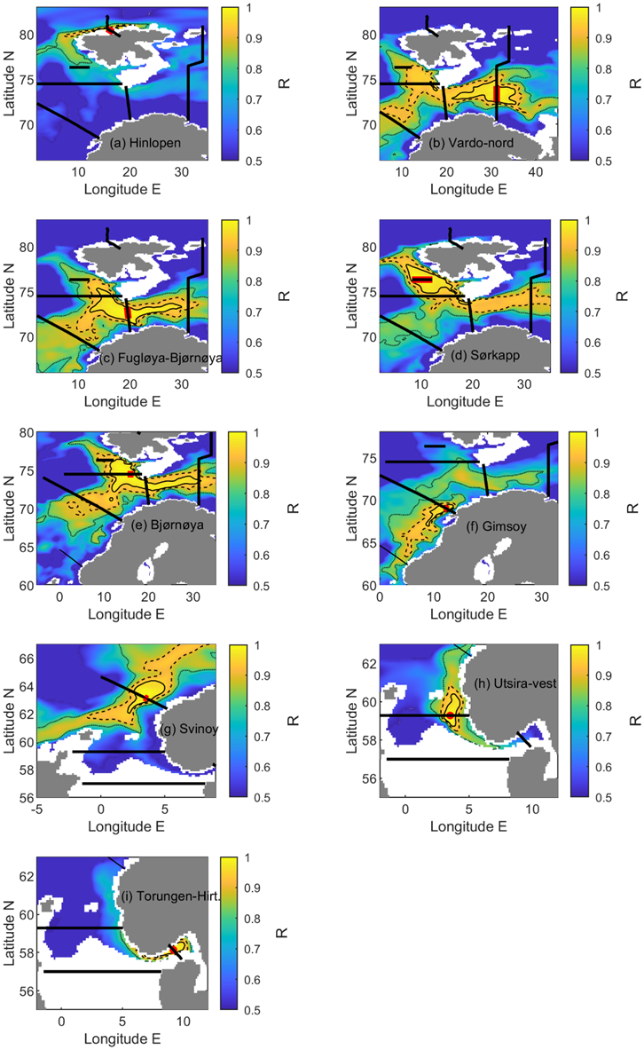
Correlation length scales indicate the spatial scales over which environmental variables covary. Maps of correlation coefficients have been used in several previous publications to provide a qualitative description of transport pathways and to assess the timescales associated with the propagation of a signal between locations (e.g. Koul et al., 2021 and Langehaug et al., 2021). Correlation length-scales can be estimated from 2-dimensional time series (for example modelled annual mean maps of temperature at a defined depth level). Correlation coefficients are calculated between one grid-point or region on a map (location-a) and all other grid-points. The resulting correlation map shows the extent to which location-a covaries with all other points in the domain. Correlation maps of this type can be used to aid the design of sampling strategy or, as here, to assess how well an existing sampling strategy captures the spatial variability in variables of interest.

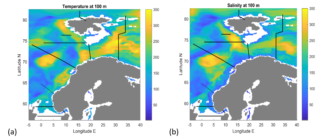
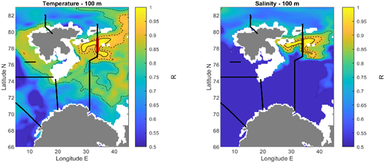
Yearly mean (1991-2021) time series of temperature and salinity fields from TOPAZ have been used to determine correlation length scales of temperature and salinity at the surface and at 100 m depth. For each of the 10 fixed CTD transects conducted by IMR, correlation maps have been generated between the grid point (or grid points) located within the core of the Atlantic Water transport pathways and all surrounding model grid points (Figs. 19-22). To identify the location of Atlantic Water transport pathways in TOPAZ, we consulted long term (1991-2021) mean current and salinity maps from the model. We then selected 1-4 grid points along each CTD transect located within the path of the strongest currents and maximum salinity. The selected grid points from the model are fairly close to the location of the stations along the CTD transect that are used for estimating Atlantic Water, although some discrepancies are present due to the model topography not being exact.

Two additional correlation plots have been generated from the 100 m temperature and salinity time series, showing the total area adjacent to each individual grid point over which time series are correlated with an R value of more than 0.95 (Figs. 23). Plots such as these indicate, for example, where moorings should be placed in order to capture conditions most representative of the surrounding region.

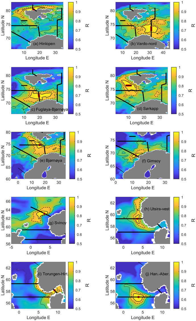
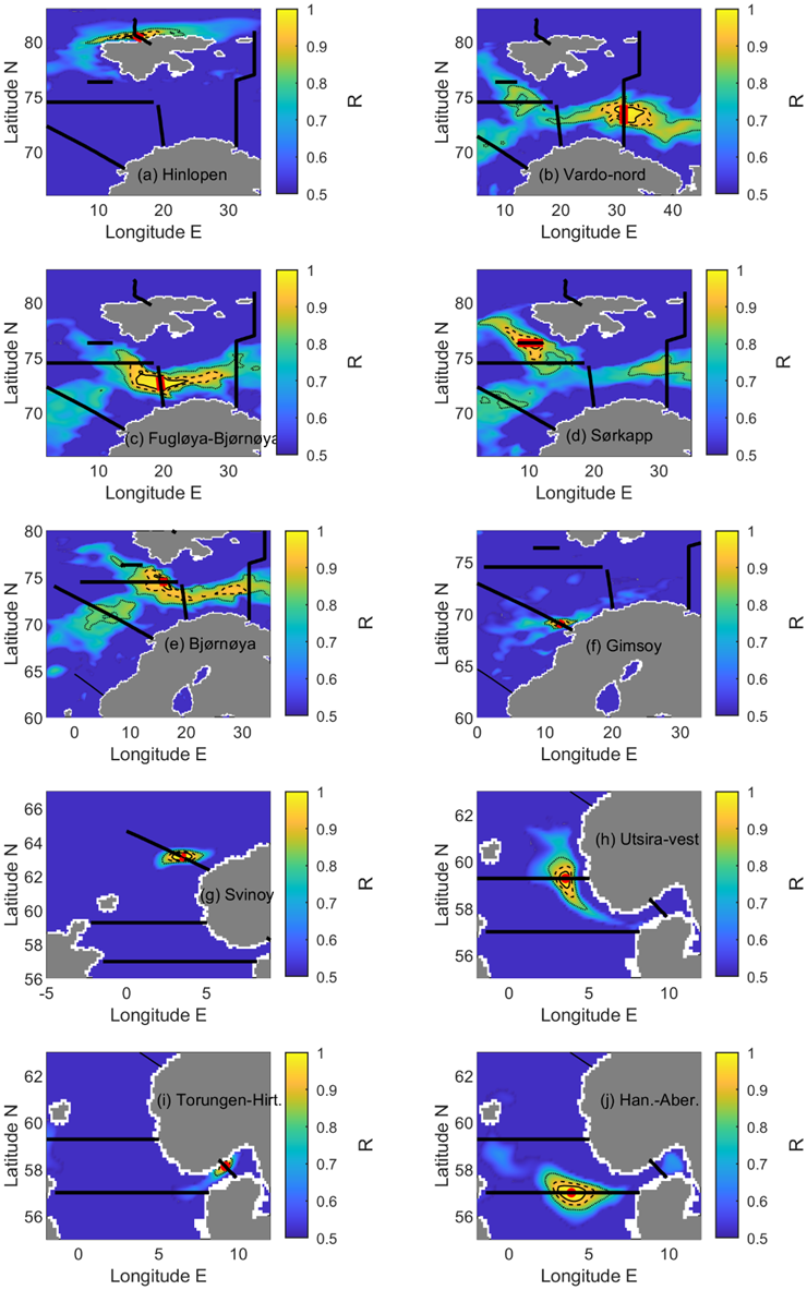
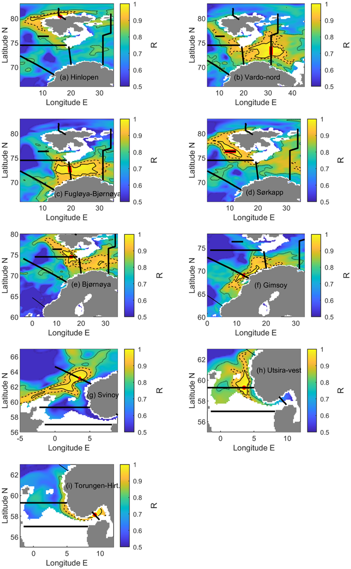
Correlation length scales vary considerably with region, depth and variable of interest and so it is important to consider the research question of interest when interpreting the correlation maps. Here we are interested in the extent to which temperature and salinity covary between adjacent transects. Correlation length scales for temperature are somewhat shorter at the surface (Fig. 19) than at 100 m depth (Fig. 21), although it is possible to detect transport pathways in the surface temperature correlation maps. Correlation length scales for salinity are considerably shorter at the surface (Fig. 20), than at 100 m depth (Fig. 22) as may be expected due to the greater influence of surface fluxes (precipitation and river runoff) and, in the north of the domain, ice dynamics. The correlation maps clearly reveal the advective transport of heat and salinity, particularly along the Atlantic inflow pathways to the Barents Sea and the Arctic Ocean, and possibly Polar Front dynamics in the Barents Sea.

In can be seen in Figs. 19-22 that there is almost no overlap of the R=0.85 contour between adjacent transects in the North Sea and the southern Norwegian sea (these being Svinøy, Utsira-West, Torungen-Hirtshals and Hanstholm-Aberdeen). The only exception being Torungen-Hirtshals which exhibits significant (R>0.9) temperature (but not salinity) co-variability with the easternmost grid points of Utsira-West. As there is little co-variability between the four southernmost transects, cutting any of them from the annual monitoring programme would be of considerable loss to long-term monitoring efforts. There is also little overlap in correlation between the Svinøy and Gimsøy sections.

There is, however, significant (R=0.9) overlap in co-variability of temperature and salinity in the northern Norwegian Sea and southern Barents Sea region, in particular for the Bjørnøya-West, Sørkapp, Fugløya-Bjørnøya, and Vardø-Nord sections. The eastern part of Bjørnøya-West, which has Sørkapp to the north, Svinøy to the south and Fugløya-Bjørnøya to the southeast exhibits significant (R>0.9) co-variability in salinity and temperature with the other sections and does not represent variability in regions not covered by the other sections. This co-variability is evident for temperature at the surface and at 100 m depth, and for salinity at 100 m depth. Thus, when focusing only on annual Atlantic Water characteristics, the Bjørnøya-West time series can be constructed based on the adjacent transects. Several provisions are, however, attached to this statement. Firstly, we have focused on assessing how well the fixed transects describe the advective transport of Atlantic influenced water towards the Arctic and have therefore focused on the eastern portion of the Bjørnøya-West section, where the Atlantic Water is concentrated. Correlation maps centred on the western sections of the Bjørnøya-West transect (Fig. 24) show that correlation length scales become smaller towards the western end of the transect. While interannual variability in temperature and salinity in the eastern reaches of the Bjørnøya-West transect are well represented by adjacent transects, variability in the western reaches of the transect is not. Bjørnøya-West extends far into the deep waters in the west and is essential for monitoring changes in the deep Greenland Basin. To assess this relevance, the co-variability of the deep western part of the Bjørnøya-West section must be compared to the corresponding deep western part of the Gimsøy section. Such a study should preferably be based on observations, as a high degree of precision is necessary due to low variability in the deep waters. Also, TOPAZ has not been evaluated for the deep basins. Secondly, we consider only how well adjacent transects covary with regard to interannual variability. If focusing on winter variability, the correlation maps and associated results would likely show a narrower correlation length scale, due to substantial mixing and heat loss during that season. Thirdly, we do not account for the considerable historical value of the data collected at this site (noting that hydrographic timeseries of multi-decadal duration are relatively rare across the globe).

There is also some overlap (R=0.9) in co-variability of temperature and salinity in the regions covered by the main Atlantic Water inflow in Fugløya-Bjørnøya and Vardø-Nord sections. Thus, focusing only on annual Atlantic Water characteristics in the southern Barents Sea, the Vardø-Nord time series can be constructed based on Fugløya-Bjørnøya. However, the co-variability patterns for temperature at surface and 100 m depth from Vardø-Nord (Figs. 19 and 21) extend further east and north in the Barents Sea as compared to Fugløya-Bjørnøya. Thus, if time series for Vardø-Nord are constructed based on Fugløya-Bjørnøya, they will not be representative of the central Barents Sea. Furthermore, as for Bjørnøya-West, the (extended) Vardø-Nord section is important for monitoring beyond the advective transport of Atlantic influenced water towards the Arctic. The section also covers the northern part of the Barents Sea (in late summer), and correlation maps centred on this part show lower correlation length scales and no overlap with other sections (Fig. 25). Thus, the extended Vardø-Nord sampling in late summer is important for monitoring the Arctic part of the Barents Sea and is more essential for monitoring than sampling of the southern part in winter.

The Hinlopen section shows no overlap in co-variability with the other sections but has a fairly wide co-variability pattern covering both the shelf and slope region north of Svalbard. Thus, it is the only section representing these waters, and it represents both Atlantic Water and more coastal waters of the northern Svalbard shelf.

In this report, we considered three numerical models developed and/or intensively used by scientists in the Oceanography and Climate Research Group; TOPAZ, Norkyst and NEMO-NAA10 km. We focused mainly on TOPAZ since this is the only of the models which both cover the entire region of interest, is fully operational and includes an ocean reanalysis. The main goal of the report was to evaluate how the model can assess and support the shipboard monitoring on our standard transects.

The version of TOPAZ assessed here assimilate CTD data, including the transects from IMR that we evaluate the model towards. It could be argued that ideally, the model should be evaluated towards an independent observational data set. This is particularly relevant if the goal is to assess if the numerical model can replace in situ sampling. However, our goal was to assess how the model can be used to support the in situ sampling and to assess sampling strategy, and earlier studies have shown that adding observations into TOPAZ in general increase the skill in reproducing the observations (Lien et al., 2016). Moreover, data that are rather sparse in time and space will have a limited effect on the increments used in the data assimilation. Based on this, we concluded that TOPAZ with data assimilation is most relevant, despite being dependent on the observations we assess. We also note that our assessment of the current velocities in TOPAZ is conducted towards an independent data set, as current measurements are not assimilated into TOPAZ. 

The assessment resulted in the following conclusions:

•    Interannual variability and multiannual trends in temperature and salinity are well represented by TOPAZ. No trend in temperature or salinity bias can be detected, suggesting TOPAZ is suitable for trend analysis. 
•    Absolute temperature and salinity values are less well represented by TOPAZ, likewise for seasonal variability and extreme conditions. TOPAZ is not considered suitable for assessing variability at seasonal or sub-seasonal timescales. 
•    TOPAZ is not suitable for the assessment of ocean currents which are typically less than 50% of those observed. However, variability in ocean currents is well represented by the Norkyst model, although currently model data are only available for a limited period (2012-today).
•    A quantitative assessment of the impact of sampling frequency on long term monitoring in the Fugløya-Bjørnøya transect suggests a minimum sampling frequency of 3-4 transects per year to prevent loss of information relating to interannual variability and trends in hydrography. A similar approach can be conducted also on the other transects. However, a full assessment of the impact of sampling frequency must include also chemical and plankton observations and models, as well as the need of capturing short-term variations like the seasonal cycle. 
•    A qualitative assessment of correlation length scales suggests the current sampling strategy is well designed in terms of the horizontal spacing of the fixed transects. However, particularly in the northern Norwegian Sea and southern Barents Sea (Sørkapp, Bjørnøya-West and Fugløya-Bjørnøya sections), the sections show a significant co-variability of Atlantic Water towards the Arctic Ocean.
•    The longest sections (Gimsøy, Bjørnøya-West and Vardø-Nord) are essential for monitoring central basin water masses in addition to the inflowing Atlantic Water. Assessing the monitoring of the deep Norwegian and Greenland basins should preferably be based on observations, as a high degree of precision is necessary due to low variability in the deep waters.
•    It is important to note that as most of the CTD data from IMR, including the transects, are assimilated into TOPAZ, a reduction in the temporal or spatial coverage of CTD monitoring might have a negative effect on the quality of the model results.
 

Albretsen, J., Sperrevik, A., Staalstrøm, A., Sandvik, A. and Vikebø, F. 2011. Norkyst800 report no. 1: User manual and technical descriptions. Technical Report 2, Fisken og Havet, Institute of Marine Research

Asplin, L., Albretsen, J., Johnsen, I.A. et al. The hydrodynamic foundation for salmon lice dispersion modeling along the Norwegian coast. Ocean Dynamics 70, 1151–1167 (2020). https://doi.org/10.1007/s10236-020-01378-0

Haidvogel, D., Arango, H., Budgell, W., Cornuelle, B., Curchitser, E., Lorenzo, E.D., Fennel, K., Geyer, W., Hermann, A., Lanerolle, L., Levin, J., McWilliams, J., Miller, A., Moore, A., Powell, T., Shchepetkin, A., Sherwood, C., Signell, R., Warner, J., and Wilkin, J. (2008) Ocean forecasting in terrain-following coordinates: Formulation and skill assessment of the Regional Ocean Modeling System. J Comput Phys 227(7): 3595–3624, predicting weather, climate and extreme events. https://doi.org/10.1016/j.jcp.2007.06.016.

Hordoir, R., Skagseth, Ø., Ingvaldsen, R. B., Sandø, A. B., Löptien, U., Dietze, H., et al. (2022). Changes in Arctic stratification and mixed layer depth cycle: A modeling analysis. Journal of Geophysical Research: Oceans, 127, e2021JC017270. https://doi. org/10.1029/2021JC017270.

Ingvaldsen, R. B., L. Asplin, and Loeng, H. (2004), Velocity field of the western entrance to the Barents Sea, J. Geophys. Res., 109, C03021, doi:10.1029/2003JC001811.

Ingvaldsen, R. (2020) Mooring data from the Barents Sea Opening – Atlantic Water inflow https://doi.org/10.21335/NMDC-1838527821

Koul, V., Sguotti, C., Årthun, M., Brune, S., Dusterhus, A., Bogstad, B., Ottersen, G., Baehr, J., and Schrum, C., (2021). Skilful prediction of cod stocks in the North and Barents Sea a decade in advance. Communications Earth & Environment. 10 pages.

Langehaug, H.R., Ortega, P., Counillon, F.S.; Matei, D., Maroon, E.A., Keenlyside, N.S., Mignot, J., Wang, Y., Swingedouw, D., Bethke, I., Yang, S., Danabasoglu, G., Bellucci, A., Ruggieri, P., Nicoli, D., and Årthun, M. (2021). Propagation of Thermohaline Anomalies and Their Predictive Potential along the Atlantic Water Pathway. Journal of Climate. 2111-2131

Lien, V.S., Hjøllo, S.S., Skogen, M.D., Svendsen, E., Wehde, H., Bertino, L., Counillon, F., Chevallier, M., and Garric, G. (2016) An assessment of the added value from data assimilation on modelled Nordic Seas hydrography and ocean transports, Ocean Modelling, 99, https://doi.org/10.1016/j.ocemod.2015.12.010.

Copernicus Marine Service, (2023) Quality Information Document, Arctic – Monitiring Forecast Centre ARCTIC_ANALYSISFORECAST_PHY_002_001, Issue 1.0.

Shchepetkin A.F., and McWilliams J.C. (2005) The regional oceanic modeling system (ROMS): a split-explicit, free-surface, topography- following- coordinate oceanic model. Ocean Model 9(4):347–404. https://doi.org/10.1016/j.ocemod.2004.08.002.

Yumruktepe, V. Ç., Samuelsen, A., and Daewel, U.: ECOSMO II(CHL): a marine biogeochemical model for the North Atlantic and the Arctic, Geosci. Model Dev., 15, 3901–3921, https://doi.org/10.5194/gmd-15-3901-2022, 2022.

8.1 - Appendix 1: Model domains

Figures A1-A3 illustrate the domain and bathymetry of each of the three models referred to in this report.

8.2 - Appendix 2: Seasonal distribution of in-situ data during each year

The number of times each of the fixed CTD transects has been conducted during a year and the seasonal spread of the data has varied considerable over time, particularly during the early part of the record. Figures A4-A6 indicate the seasonal spread of data during each year of occupation along Bjørnøya-Fugløya, Svinøy, and Utsira-West.

8.3 - Appendix 3: Seasonal variability along transects

8.4 - Appendix 4: BSO mooring programme

Velocity data collected by current meters situated along a north-south transect across the Barents Sea Opening have been used to assess the performance of the models in reproducing observed velocities in this region. Table 2 details the data availability between 1998 and 2017.

Table 2: Details of the Barents Sea Opening mooring programme. Further details can be found in Ingvaldsen et al. (2004).

8.5 - Appendix 5: Comparison of CTD station locations and TOPAZ model grid points

The CTD stations are overlain on the TOPAZ model grid in Figures A7-A9 in order to illustrate how the horizontal resolution of the TOPAZ model compared to that of the CTD stations.

HAVFORSKNINGSINSTITUTTET

Postboks 1870 Nordnes

5817 Bergen

Tlf: 55 23 85 00

E-post: post@hi.no

www.hi.no