Report series:
IMR-VNIRO 2026-7Published: 06.10.2026Project No.: 16150On request by: IMR/VNIRO Program:
Barentshavet og Polhavet Approved by:
Research Director(s):
Geir Huse
Program leader(s):
Maria Fossheim
Summary
The aim of the joint Norwegian/Russian ecosystem survey in the Barents Sea and adjacent waters, August-October (BESS) is to monitor the status and changes in the Barents Sea ecosystem and provide data to support stock advice and research. The survey has since 2004 been conducted annually in the autumn, as a collaboration between the Institute of Marine Research (IMR) in Norway and the Polar branch of the VNIRO (PINRO) in Russia. The general survey plan and tasks were agreed upon at the annual IMR-PINRO Meeting in March 2024. Ship routes and other technical details are agreed on by correspondence between the survey coordinators. BESS aims at covering the entire Barents Sea. Ecosystem stations are distributed in a 35×35 nautical mile regular grid, and the ship tracks follow this design. Exceptions are the area around Svalbard/Spitsbergen, some additional bottom trawl hauls for demersal fish survey indices estimation, and additional acoustic transects for the capelin stock size estimation.
The 22-th BESS was carried out during the period from 22. August to 15. October by the Norwegian research vessels “Helmer Hanssen”, “G.O. Sars” and “Johan Hjort”, and the Russian vessels “Vilnyus”.
As always, we would like to express our sincere gratitude to all the crew and scientific personnel onboard RVs “Vilnyus”, “G.O. Sars”, “Helmer Hanssen” and “Johan Hjort” and for their dedicated work, as well as all the people involved in planning and reporting of BESS 2025.
The information obtained in BESS 2025 will be further used for the implementation of various international and national projects, assessment of fish and invertebrate stocks, environmental monitoring, etc.
1 - Background
Author(s):
Geir Odd Johansen
(IMR) and Dmitry Prozorkevich (VNIRO-PINRO)
The aim of the Barents Sea ecosystem survey (BESS) in August-October is to monitor the status and changes in the Barents Sea ecosystem. The survey has been conducted annually since 2004, as collaboration between the IMR in Norway and the Polar Branch of VNIRO (PINRO) in Russia. The general survey plan, tasks, and sailing routes are usually agreed upon at the annual PINRO-IMR Scientists’ Meeting in March. From 2024, the meeting has gone digital due to external factors. The 22nd BESS was carried out during the period from 22nd August to 15th October 2025 by the Norwegian research vessels (“Helmer Hanssen”, “G.O. Sars” and “Johan Hjort”) and the Russian vessel (“Vilnyus”). The scientists and technicians taking part in the survey onboard the research vessels are listed in Table 1. As always, we would like to express our sincere gratitude to all the crew and scientific personnel onboard the research vessels for their dedicated work. We would also express our sincere gratitude to all the people involved in planning and reporting of BESS 2025.The purpose of this survey report is to summarize the status of the environmet and the living organisms of the Barents Sea based on the survey data. The information obtained in BESS 2025 will be further used for the assessment of fish and invertebrate stocks, the evaluation of changes in environmental conditions and biota, and the implementation ov various international and national projects.
Table 1. Vessels and participants (with main expertise) in the Barents Sea Ecosystem Survey 2025.
Rupert Wienerroither (Cruise leader), Erlend Lindau Langhelle (Demersal fish), Silje Seim (Demersal fish), Åse Husebø (Demersal fish), Viggo Edvardsen (Demersal fish; 17-22.09), Lotta Lindblom (Demersal fish; 23.09-08.10), Erling Boge (Pelagic fish), Merete Kvalsund (Pelagic fish), Terje Berge (Plankton), Hege Skaar (Plankton), Jarle Kristiansen (Instrumentation), Sebastian Grieg Pedersen (Instrumentation), Deanna Leonard (Marine mammals observer), George McCallum (Marine mammals observer), Håvard Eggen (Sea birds observer; guest; NINA), Penny Lee Liebig (Benthos), Robert Andre Johansen (Benthos), Hans Dybvik (Instrumentation; 17-23.09; guest; UiT), Markus Opdal (Instrumentation; 17.-23.09; guest; UiT), Ronald Berntsen (Instrumentation; 23.09-08.10; guest; UiT), Carl Ballantine (Instrumentation; 23.09-08.10; guest; UiT)
”G.O. Sars” (31.08–27.09)
Part 1 (31.08-08.09)
Arved Staby (Cruise leader), Anne Kari Sveistrup (Benthos), Olaf J. Sørås (Instrumentation), Hege Haraldsen Lien (Demersal fish), Irene Huse (Demersal fish), Erlend Lindau Langhelle (Demersal fish), Sigmund Grønnevik (Demersal fish), Stine Karlson (Pelagic fish), Lea Marie Hellenbrecht (Pelagic fish), Marianne Petersen (Plankton), Mona Ring Kleiven (Plankton), Josefina Johansson (Benthos), Birgitta Mueck (Marine mammals observer), Claudia Erber (Marine mammals observer), Sverre Waardal (Instrumentation), Marte Elise Rørsdtad (Student; guest; UiB)
Part 2 (10.09-27.09)
Anne Kristine Frie (Cruise leader), Anne Kari Sveistrup (Benthos), Tor Ensrud (Benthos), Olaf J. Sørås (Instrumentation), Anne Margrethe Aase (Demersal fish), Janicke Skadal (Demersal fish), Halvard Aas Midtun (Demersal fish), Markus Skadal (Demersal fish), Eilert Hermansen (Pelagic fish), Adam Custer (Pelagic fish), Ann-Kristin Olsen (Plankton), Linda Fonnes Lunde (Plankton), Thomas André Sivertsen (Marine mammals observer), Lars Kleivane (Marine mammals observer), Jon Arild Aarsborg (Instrumentation), Eli Gustad (Plankton), Eli Inntveit (Student; guest; UiB), Erik Grønningsæter (Sea birds observer; guest; NINA)
Hector Pena (Cruise leader), Tommy Gorm-Hansen Tøsdal (Pelagic fish), Rune Strømme (Instrumentation), Yasmin Hunt (Marine Mammal observer), Frederike Boehm (Marine Mammal observer), Fredrik Gelin (Instrumentation), Erling Boge (Pelagic fish), Elena Eriksen (Scientist; ecology), Guosong Zhang (Scientist; acoustics), Marte Louise Strømme (Instrumentation), Babak Khodabandeloo (Scientist; acoustics), Gary Elton (Sea birds observer; guest; NINA), Ricco Ip (Student; guest; UiB).
Part 3 (16.09-09.10)
Georg Skaret (Cruise leader), Andrey Voronkov (Benthos), Yasmin Hunt (Marine Mammal observer), Frederike Boehm (Marine Mammal observer), Fredrik Gelin (Instrumentation), Else Holm (Demersal fish), Vidar Fauskanger (Demersal fish), Atle Børje Rolland (Demersal fish), Frøydis Tousgaard Rist (Pelagic fish) Aina Bruvik (Pelagic fish), Timo Meissner (Pelagic fish), Jon Rønning (Plankton), Jane Strømstad Møgster (Plankton), Monica Martinussen (Benthos), Trond Bjordal (Instrumentation), Jon Ford (Sea birds observer; guest; NINA)
2 - Survey Execution
Author(s):
Geir Odd Johansen
(IMR) and Dmitry Prozorkevich (VNIRO-PINRO)
Figures by: Stine Karlson
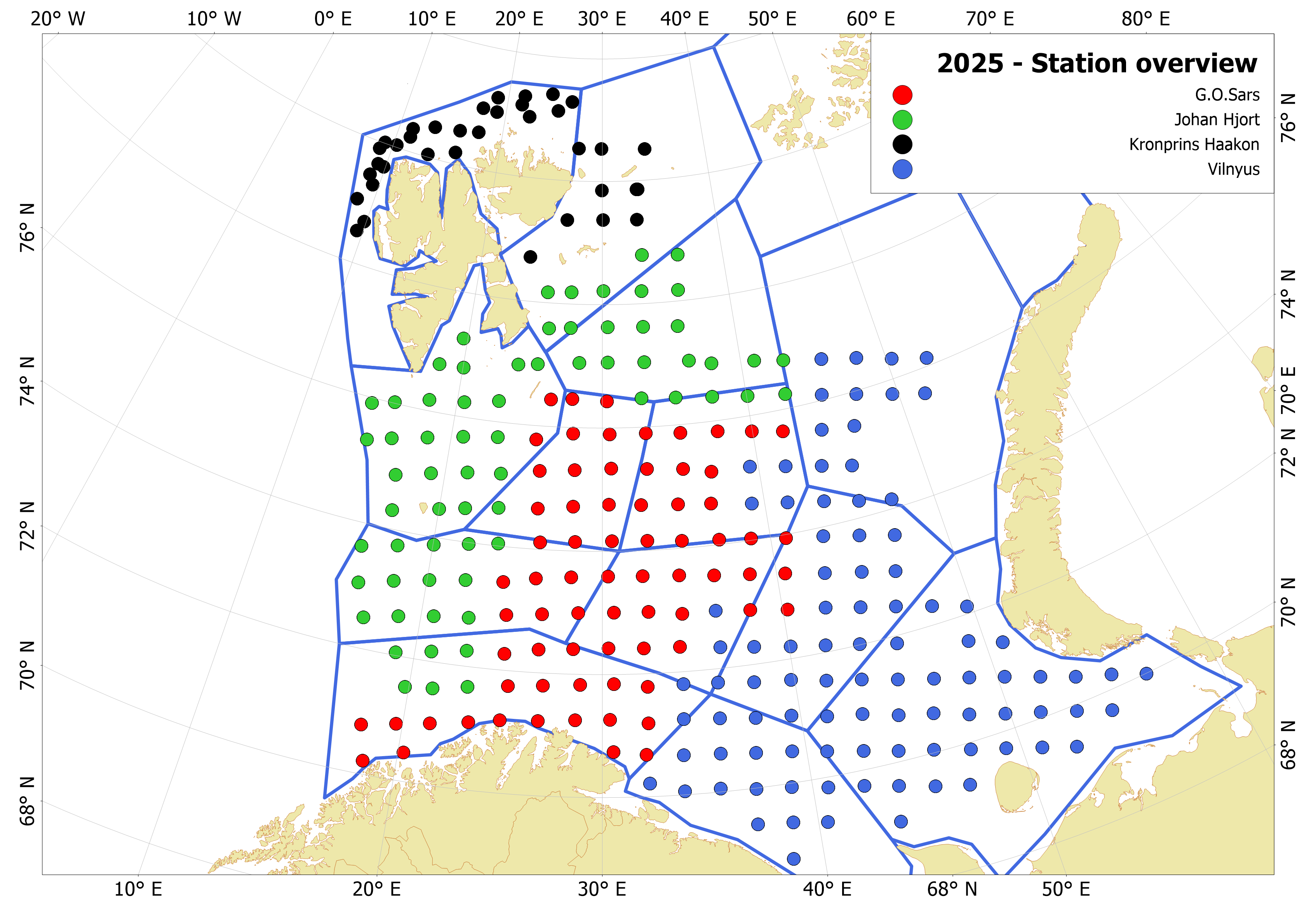
BESS aims at covering the entire, ice-free area of the Barents Sea, progressing from south to north. Ecosystem stations are distributed in a 35×35 nautical mile regular grid, and the ship tracks follow this design. Exceptions are the areas west and north of Svalbard/Spitsbergen, where the tracks follow a zig-zag design where depth stratified (100-300m and 300-500 m) bottom trawl hauls for demersal fish survey indices estimation are distributed along the tracks. There are also additional acoustic transects between the tracks covering the ecosystem stations east of Svalbard/Spitsbergen, and south of Franz Joseph Land, to increase the overage for acoustic capelin stock size estimation. This constitutes a standard plan for the survey.
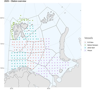
The planned vessel tracks for BESS 2025 are given in Fig. 2.1. The plan for the Norwegian vessels had to be changed relative to the standard plan due to issues with the time allocation between Norwegian vessels. Due to this, we had to plan for a later coverage by “G.O. Sars” part 2 of the areas between Bear Island and Svalbard/Spitsbergen, as well as a central part of the Norwegian Exclusive Economic Zone (NEEZ). BESS 2025 was largely implemented according to this modified plan.
Figure 2.1. BESS 2025 planned survey map with ecosystem stations and vessel tracks.
The Russian RV “Vilnyus” covered the eastern and north-eastern parts of the Barents Sea within the Russian Exclusive Economic Zone (REEZ), as well as bottom trawls in the Russian shelf part of the Loophole. Norwegian RVs covered the western part of the Barents Sea and an area around Svalbard/Spitsbergen within the NEEZ, as well as pelagic samples in the Russian shelf part of the Loophole. More specific, “Johan Hjort” covered the western part of the NEEZ south of Bear Island, as well as the areas west of Svalbard/Spitsbergen in NEEZ, which is part of the capelin feeding area. “G.O. Sars” covered the eastern part of NEEZ, and the central parts according to the modified plan. “Helmer Hanssen” covered the areas west, north, and north-east of Svalbard/Spitsbergen. The realized research vessel tracks with sampling for the BESS 2025 are shown in Figs. 2.2 and 2.3. Exceptions to the planned coverage were one missed station in the central NEEZ due to time constraints, and a larger area west of Novaya Zemlya in REEZ where only acoustic transects were carried out, because trawls operations are prohibited in this area.
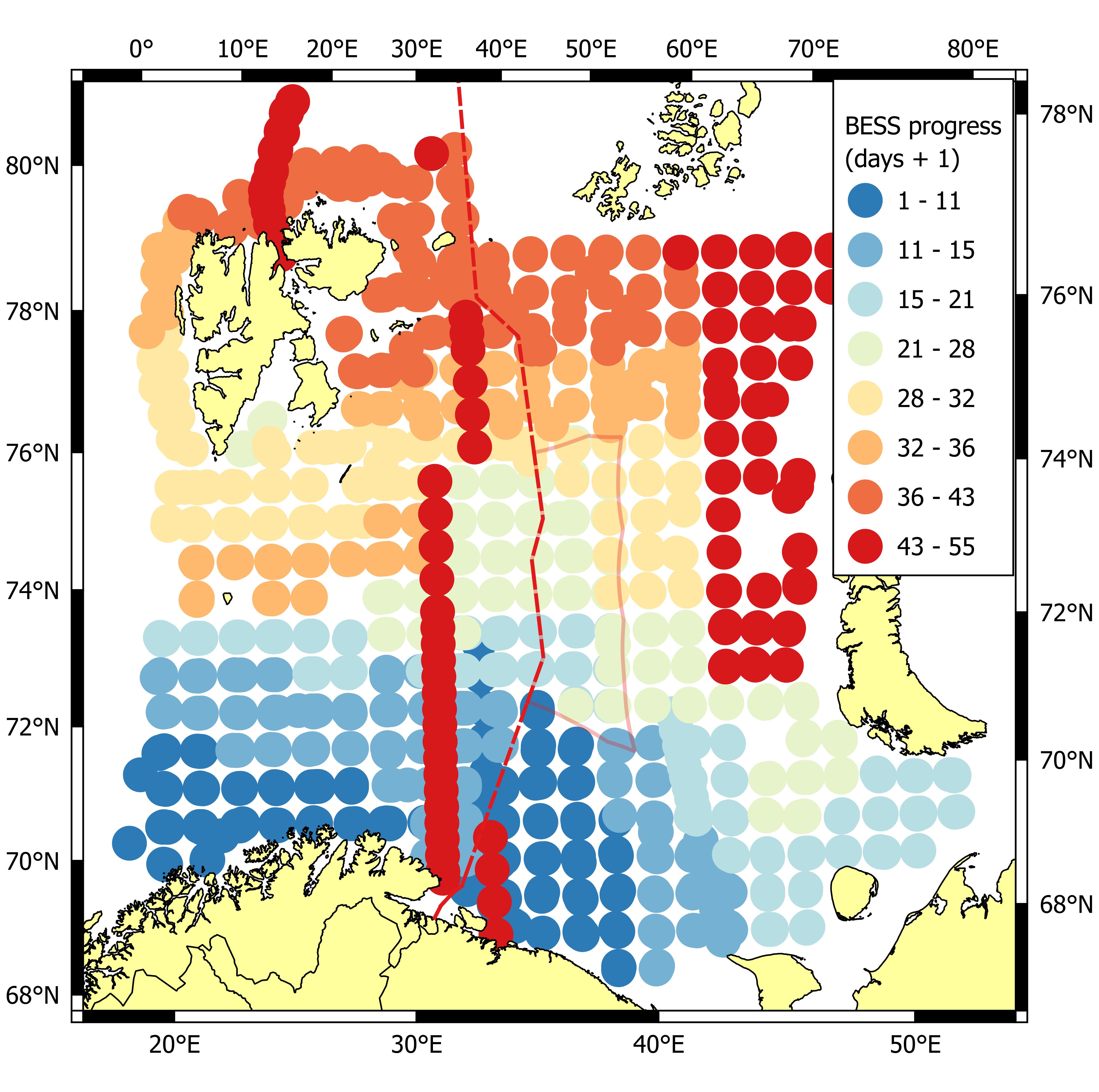
The planned time schedule for BESS 2025 was 155 days (100 NOR+55 RUS), while the effective vessel days (time between first and last sample in the vessel logs) was 141 days (89 NOR+52 RUS). The difference between the two is as expected, as vessels need time for sailing to and from harbours, some preparation before sampling at stations, and due to incidents of bad weather. The overall temporal and spatial progression during the survey was according to the ideal southwest to northeast progression (Fig. 2.4). An exception due to the later coverage by “G.O. Sars” part 2 of the areas between Bear Island and Svalbard/Spitsbergen, as well as a central part of the NEEZ is visible.
Figure 2.2. BESS 2025, realized vessel tracks with pelagic and bottom trawl stations, note that some trawl stations are taken in addition to the regular ecosystem stations.
Figure 2.3. BESS 2025 realized vessel tracks with hydrography, plankton and other samples.
Figure 2.4. Progression of BESS 2025 in space and time. Points represent samples taken at ecosystem stations during the survey. The point colouring indicates the number of days between the start date of the survey and sample date (+1). The colours scale from blue (early in the survey) to red (late in the survey).
2.1 Sampling methods
The ecosystem survey in 2025 was like previous years, covering most ecosystem components. In addition, the standard oceanographic sections "Vardø-Nord" and "Hinlopen" were taken by the Norwegian vessels, and the “Kola” (twice) and Kanin sections were taken by the Russian vessel (Fig. 2.3). Summarizing the standard sampling gears at the BESS 2025; in total 311 pelagic hauls, 354 demersal hauls, 432 CDT, and 430 plankton nets were taken.
In 2025, compared to 2024, there were no changes in sampling gear. Manta trawl was included as standard equipment for monitoring microplastics at BESS in 2022 and was also used in 2025. 50 Manta samples were collected on the Russian vessel, and 38 on board the Norwegian vessels. In addition, 34 fish stomachs were sampled on the Russian vessel for the same purpose.
A new length stratified individual sampling of haddock was introduced in 2022, increasing samples from one to two fish taken per 5 cm group. This continued in 2025.
Plankton stations were carried out throughout the entire area covered by the survey with sampling from surface to bottom. On the Kola hydrological section, plankton samples are collected separately for the layers: 0-50 m, 0-100 m and 0 to bottom.
The survey sampling manuals can be obtained by contacting the survey coordinators. These manuals include methodological and technical descriptions of equipment, the trawling and capture procedures by the sampling tools, sampling and registration of the ctach in the lab, and the methods thatbare used for calculating the abundance and biomass of biota.
2.2 Special investigations
BESS is a useful platform for conducting additional studies in the Barents Sea. These studies can be testing of new methodology, sampling of data additional to the standard monitoring, or sampling of other types of data. It is imperative that the special investigations do not influence the standard monitoring activities in the survey. The special investigations vary from year to year and below is a list of special investigation conducted on Russian and Norwegian vessels at BESS 2025, with contact persons. This chapter also briefly mentions some investigations that are typical during survey but not described in the main text of the BESS Report.
2.2.1 Annual monitoring of pollution levels
In 2025 PINRO continued the annual monitoring of pollution levels in the Barents Sea in accordance with a national program. Samples of seawater, sediments, fish and invertebrates were collected and analyzed for persistent organic pollutants (POPs, e.g. PCBs, DDTs, HCHs, HCB) and heavy metals (e.g. Pb, Cd, Hd) and As. The samples were collected at RV "Vilnyus" during BESS in different parts of the Barents Sea. The results from chemical analyses are available in the annual PINRO report “Status of biological resources…”.
2.2.2 Collection of samples for biochemical studies
Frozen samples of commercial and non-commercial fish and invertebrates were collected for biochemical studies (ratio of body parts, chemical composition of nutrients, molecular weight of muscle proteins, amino acids and lipid fractions composition) in accordance with a research program. Samples were frozen at temperature -18°C immediately after catching before rigor mortis.
Contact: Kira Rysakova, PINRO (rysakova@pinro.vniro.ru)
2.2.3 Fish pathology and parasitological research
PINRO undertakes yearly investigations of fish diseases in the Barents Sea (mainly in REEZ). Seven commercially important fish species were analyzed visually (19321 individuals) and 957 individuals for detailed parasitological analysis. In addition, red king crab and snow crab (in total 526 individuals) were examined for “shell disease of crustaceans”. The main purpose of the pathology research is annual estimation of epizootic state of commercial fish and crab species. The observations are entered into a database on pathology. This investigation was started by PINRO in 1999. Results are available in the annual PINRO report “Status of biological resources…”
In August and October, hydrochemical observations were made onboard RV “Vilnyus” in the Kola section. Dissolved oxygen in the surface and bottom layers as well as biochemical oxygen demand during 5 days in the bottom layer were measured.
Since 2004, investigations of diet of most abundant pelagic and demersal fish have been conducted annually during the BESS. Stomach samples from polar cod and capelin, and cod, are collected as standard at both Russian and Norwegian vessels, and the detailed sampling is reported in the chapters about pelagic and demersal fish, respectively.
The Russian vessel in 2025 also collected stomachs from Atlantic herring, haddock, Greenland halibut and skates (704 individuals), and snow crab (96 individuals) were fixed for detailed analysis. In addition, 4026 stomachs of 16 fish species were sampled and analyzed by “express quantitative analysis”.
In 2016 we collected eDNA (environmental DNA) samples in the North of Svalbard and the Barents Sea to test if the method can map the distribution of fish species in an easier way compared to traditional methods as conventional trawling. The eDNA is sequenced and species are identified by comparing these sequences (Barcode) against a reference database. Since 2018, we have sampled and analyzed the DNA. In the NFR project FISHDIV we have developed a method to quantify biomass of fish species (including Atlantic cod and herring) in fjords. Next step would be to test this method for fish species in the Barents Sea. The analysis of eDNA can identify all species such as marine mammals, fish and zooplankton in a drop of water. The analysis of eDNA through metabarcoding (massive parallel DNA sequencing) is an established and validated method for species identification/community analysis but has not been used routinely on expeditions in the Barents Sea. This type of DNA sample can support other sampling to monitor species composition in the Barents Sea. It is a method for the future and would be important in assisting in monitoring species distribution in relation to climate change.
Sampling of seawater from a total of 6 CTD stations, 125 l seawater taken from the sea water tap on deck. The water samples will be used for analyses and monitoring of radioactivity in seawater in the Barents Sea.
Microplankton metabarcoding samples are collected from 10 m CTD water at standard stations where time allows. Samples collected through this special investigation will be used to test a new methodology to characterize microplankton community composition, DNA metabarcoding. Metabarcoding samples will be collected on the G.O. Sars at all standard stations when possible, completing a three-year time series in the region. The standard method used to characterize microplankton communities, microscopy, is relatively expensive and can only resolve visually distinct taxa. DNA metabarcoding will complement microscopy by increasing the spatial and taxonomic resolution of our results regarding microplankton community distribution and composition. The results from this investigation can be used to inform decisions regarding the value and role of metabarcoding in Barents Sea ecosystem monitoring efforts. This work is a continuation of phytoplankton metabarcoding sampling conducted in 2022-204 and includes the collection of similar samples for 2025.
Contact: Sarah Lerch, IMR (sarah.lerch@hi.no)
2.2.9 Additional WP2 samples at 100-0m
WP2 net lowered to 100m depth and then pulled vertically up to the surface. If sufficient time is available, 100–0 m samples are desired at all plankton stations.
We apply for zooplankton sampling with WP2 net for the upper part of the water column (100-0m), which comes in addition to the sampling already established for the bottom-0m stratum. This “double sampling” is already performed along the transects, but we now wish to extend this to all plankton stations. This double sampling was standard procedure from about 1990-2014, but the sampling was thereafter limited to the bottom-0m stratum. The reason for asking to re-establish the 100-0m sampling is that this better represents the depth-habitat for young stages of fish, thereby probably being more relevant as a proxy for their ambient feeding environment than the bottom-0m stratum. That said, the bottom-0m samples are vital when assessing trends and year-to-year variation in plankton abundance as these represent the whole plankton community in the entire water column. I believe the 100-0m samples might become an additional valuable ecosystem indicator when assessing the underlying reasons for the variation in years class strengths and poor recruitment of the fish stocks in the later years. Hence, both types of samples are important, but in different ways.
2.2.10 Freeze samples of krill, amphipods, and capelin for nutrient analysis
Capelin and krill are important prey for baleen whales in the Barents Sea. In order to investigate how baleen whales assimilate nutrients during digestion, samples of capelin and krill will be analyzed for macronutrients and trace metals and later compared with nutrient contents in whale excretions. For this reason, samples of capelin and krill were taken at several relevant stations during the ecosystem cruise. In each station, a sample of 25 capelin and 50 krill were collected and stored in the freezer. This work is part of the EU project OceanICU.
Contact: Carla F. Brandt, IMR (carla.freitas.brandt@hi.no) and Martin Wiech (Martin.Wiech@hi.no)
2.2.11 Sub-samples from WP2 and MultiNet Mammoth nets for molecular analysis of zooplankton
Quantitative sub-samples will be taken from all standard zooplankton samples from WP2 and MultiNet Mammoth nets) for molecular analysis (community DNA metabarcoding). These samples (1/4 of the total sample) will be homogenized onboard and a portion of the homogenate will be preserved in TES buffer. This procedure saves significant downstream processing time in the lab and avoids the use of ethanol which presents many logistical challenges. These samples will complement traditional microscopic sorting by generating high-resolution species-level data on the zooplankton communities and allowing to process more samples than would be possible through microscopic analysis alone. This will also generate data on groups often missed by microscopy, such as cryptic species and larvae of benthic animals, including commercially and ecologically important ones, such as king- and snow crab.
2.2.12 Freeze samples of zooplankton analysis of vitamin B and lipids
Zooplankton collected from WP2-net or from demersal trawl samples are frozen at selected stations. The samples from WP2-net are fractionated using the standard method (180-1000 µm, 1000-2000 µm, for >2000 µm). When possible, we do also wish for species sorted samples (see table 1). The frozen material will be brought back to the lab in Bergen for further analysis of b-vitamin, fatty acids and stable isotope analysis.
2.2.13 Freeze samples of 0-group capelin, herring and redfish
Small juvenile 0-group herring, capelin and redfish from pelagic and demersal trawl samples are frozen at selected stations. The frozen material will be brought back to the lab in Bergen for further analysis of condition/growth, fatty acids and stable isotope analysis.
2.2.14 Freeze samples of juvenile cod and polar cod
Small juvenile cod and polar cod, mainly 0-group and some 1-group from pelagic and demersal trawl samples are frozen at selected stations. Otoliths of sampled cod will be used for two MSc projects at UiB and IMR dealing with 3 D otolith structure and relative otolith versus somatic growth. The frozen material will be brought back to the lab in Bergen for further analyses of condition and growth within the framework of an RCN-proposed project. These analyses are dependent on higher resolution of fish attributes than normally possible at sea.
A total sample of 3 kg of whole shrimp from the Barents Sea, collected anywhere in the Barents Sea, are frozen and brought on land. The sample will be used for analyses and monitoring of radioactivity in shrimp in the Barents Sea.
There is a mismatch between the generally assumed distribution of the commercially important Iceland scallop (Chlamys islandica) in the Barents Sea and Svalbard area and much more widely registered observations on the BESS. Using genetic analysis to confirm species identification and study the population structure will help to improve our understanding of the distribution of this species and links to bathymetry, habitat and environment. Up to 30 individuals per station will be collected and stored at -20C for tissue sampling, morphological analysis and ageing. The results will contribute to the stock assessment and fisheries advice for Iceland scallops in the Barents Sea and Svalbard/Spitsbergen area.
2.2.17 Acoustic target strength (TS) measurements of capelin
Fish target strength (TS) is a key parameter for abundance and biomass estimation of fish stocks when using the acoustic echo integration methods. A 5-days period on RV Johan Hjort was dedicated to obtaining acoustic data suitable for target strength measurements with a TS probe. This is a platform equipped with five echosounders (38 kHz narrowband and 70, 120, 200, and 333 kHz broadband) and transceiver tubes that can be lowered close to the targets. There were problems with the main plug between the probe and the winch cable were solved by opening the probe and using spare connectors. Unsuccessful calibration of probe echo sounders because it was impossible to obtain isolated sphere targets due to abundant fish around the sphere in the calibration site. TS probe will require permanent repair of defects and complete maintenance of all systems (including relay module and pitch/roll motors). During the survey, fish aggregations that were evaluated as capelin using the echo sounder data, were confirmed to be polar cod after trawling. Contrary, aggregations that were not considered to be capelin because of high backscattering in high frequencies, corresponded to capelin after trawling during the acoustic coverage in the capelin area after the 5-days test. The anomalous frequency response observed coincide with what was measured during surveys in the spawning period in the coast of Finnmark in February-March.
Contact: Georg Skaret, IMR (georg.skaret@hi.no) and Hector Pena (hector.pena@hi.no)
3 - Data Management
Author(s):
Geir Odd Johansen
(IMR) and Dmitry Prozorkevich (VNIRO-PINRO)
3.1 Data Bases
A wide variety of data are collected during the ecosystem surveys. All data collected during the BESS are quality controlled and verified by experts: oceanography by Randi B. Ingvaldsen (IMR) and Aleksandr Trofimov (PINRO) fish catch data by Herdis Langøy Mørk (IMR) and Tatyana Prokhorova (PINRO) during and after the survey; plankton data by Jon Rønning and Espen Bagøien (IMR) and Irina Prokopchuk (PINRO); benthos data by Anne Kari Sveistrup (IMR) and Nataliya Strelkova (PINRO); and marine mammals data by Frederike Boehm (IMR) and Roman Klepikovskiy (PINRO). The data are stored in IMR and PINRO national databases, with different formats. However, the data is exchanged so that researchers in both institutes have access to each other’s data and use equal joint data.
3.2 Data Application and reporting
The BESS aims to cover the whole Barents Sea ecosystem geographically and provide survey data for commercial fish and shellfish stock assessment. Data for stock assessment of capelin is particularly important, because capelin TAC (Total Allowable Catch quota) is specifically based on the results from this survey. The Norwegian-Russian Fishery Commission determines TAC immediately after the survey. In addition, a broad spectrum of physical variables, ecosystem components and pollution are monitored and reported, and included in other kinds of assessments, e.g. ecosystem-based assessments. The survey data will be used by each party for various purposes within the framework of national and international programs.
This survey report is based on joint data and contains the main results of the monitoring. The survey report will be published in the report series «IMR/Polar Branch of VINRO Joint Report Series.
Prior to this report, the survey reports from BESS in the period 2004 – 2025 have been published in the report series “IMR/PINRO Joint Report series”.
All reports from BESS from 2004 until the latest are available at this web site:
Author(s):
Alexander Trofimov (VNIRO-PINRO), Randi Ingvaldsen
(IMR), Tatyana Prokhorova (VNIRO-PINRO), Bjørn Einar Grøsvik
(IMR) and Roman Klepikovskiy (VNIRO-PINRO)
4.1 Hydrography
Text by: A. Trofimov and R. Ingvaldsen
Figures by: A. Trofimov
4.1.1 Geographic variation
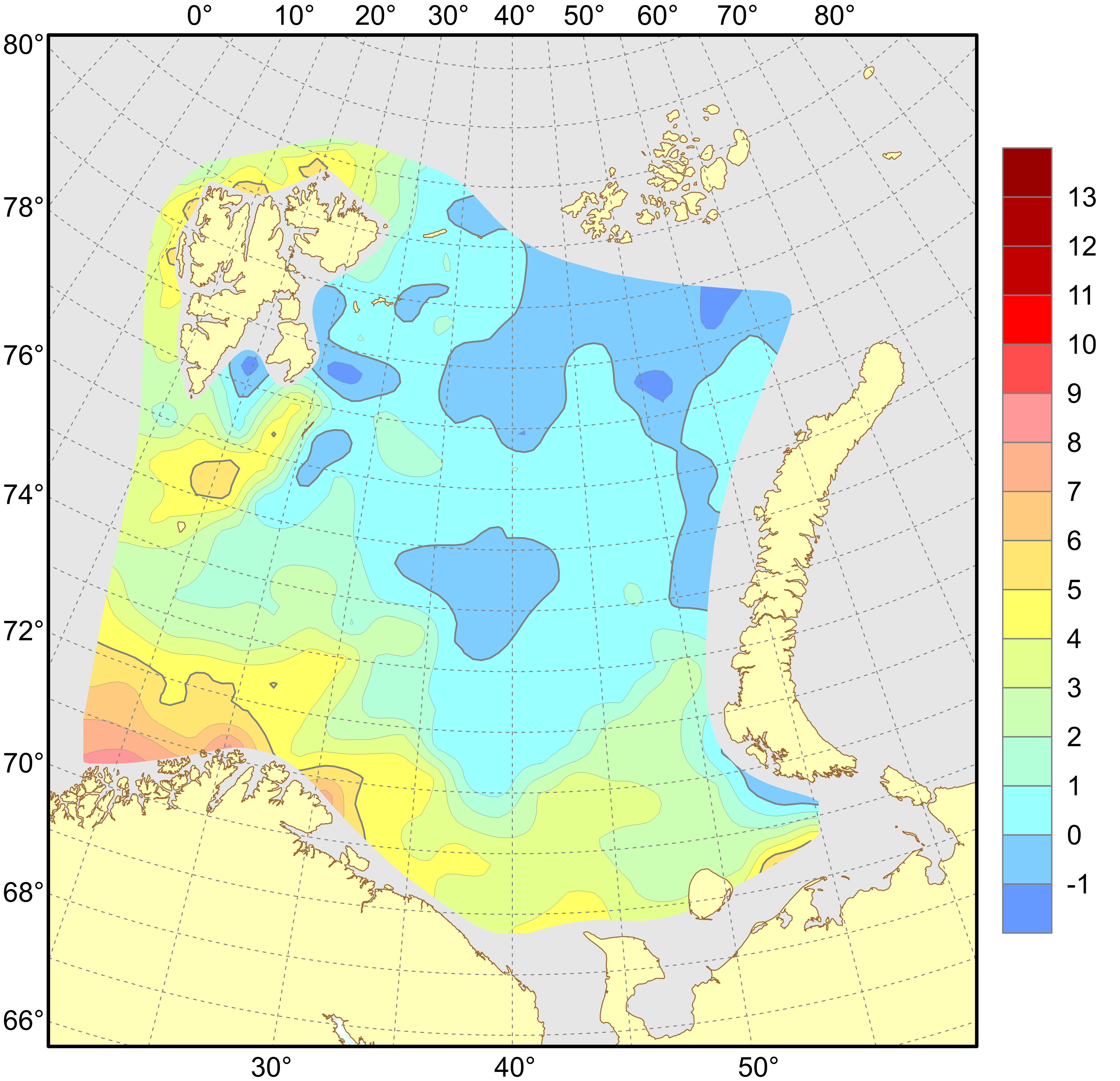
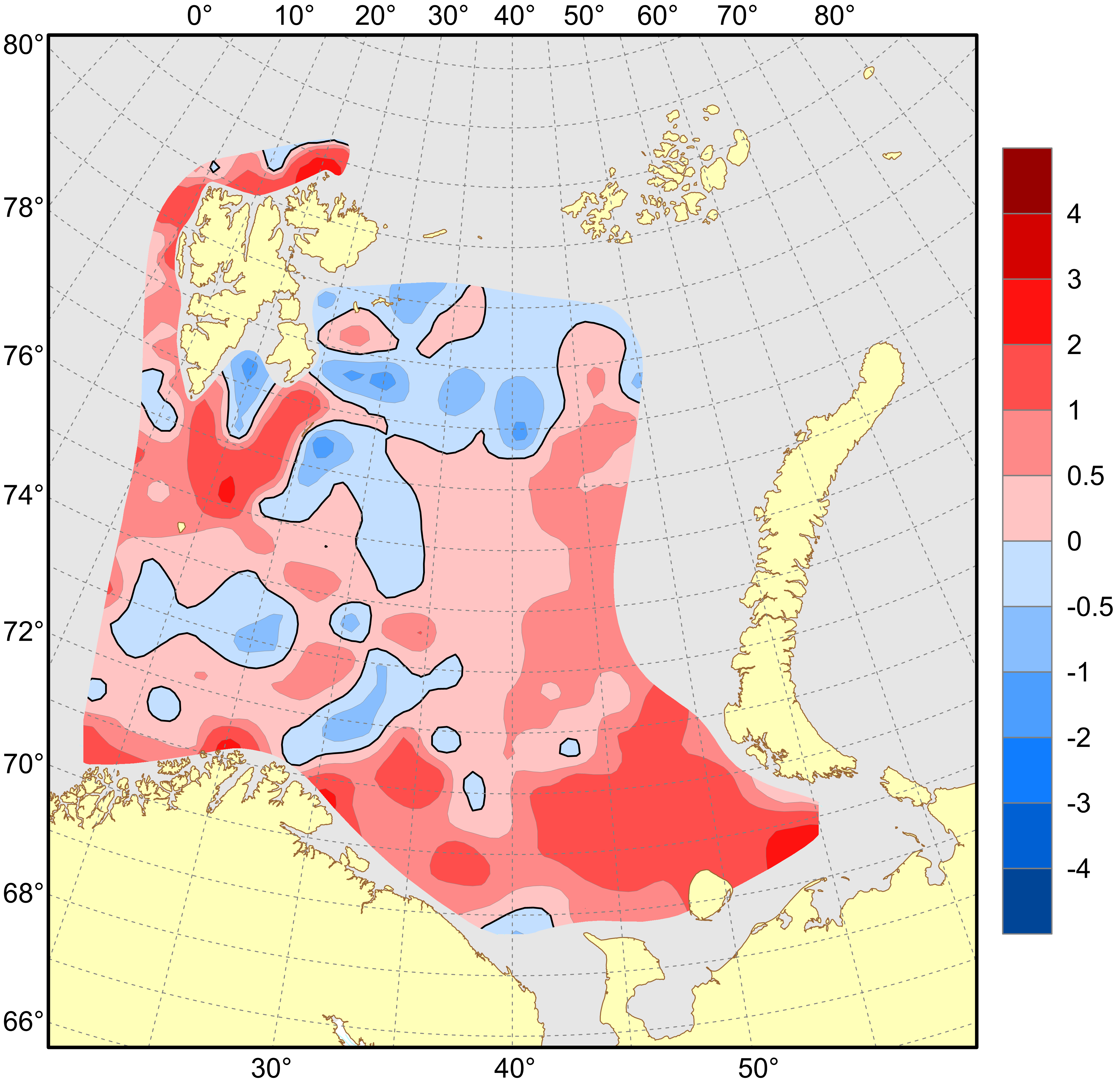
Horizontal distributions of temperature and salinity are shown for depths of 0, 50, 100 m and near the bottom in Figs 4.1.1.1–4.1.1.8, and anomalies of temperature and salinity at the surface and near the bottom are presented in Figs 4.1.1.9–4.1.1.12. The anomalies have been calculated using the long-term means for the period 1991–2020.
In August–October 2025, surface temperature was on average 1.9°C higher than the long-term mean all over the surveyed area, with the largest positive anomalies (>3°C) in the southeastern Barents Sea (Fig. 4.1.1.9). Compared to 2024, the surface temperature in 2025 was much lower (by 1.4°C on average) in most of the area (85%), with the largest negative differences (>2°C in magnitude) in the south and west. Positive differences (0.6°C on average) were mainly found in the northern and southeastern parts of the sea.
Arctic waters were mainly found, as usual, in the 50–100 m layer north of 77°N (Fig. 4.1.1.3 and 4.1.1.5). Temperatures at depths of 50 and 100 m were higher than the long-term means (on average, by 0.7 and 0.6°C respectively) in about two thirds of the surveyed area, with the largest positive anomalies (>1°C) at 50 m depth in the western, southernmost and southeastern Barents Sea. Negative anomalies (on average, −0.4°C at 50 m and −0.3°C at 100 m) were mostly found in the central part of the sea. Compared to 2024, the 50 and 100 m temperatures in 2025 were higher (on average, by 0.9 and 0.7°C respectively) in half of the surveyed area (mainly in the western, southern and southeastern parts), with the largest positive differences (>2°C) at 50 m in the southeast. Negative differences were mainly observed in the central and northern Barents Sea. Small temperature anomalies and differences between 2025 and 2024 (both negative and positive, <0.5°C in magnitude) occupied from 46 to 56% of the area.
Bottom temperature was in general 0.7°C above average in 75% of the surveyed area, with the largest positive anomalies (>1°C) mainly in the southeast (Fig. 4.1.1.10). Bottom waters in 2025 were 0.8°C warmer than in 2024 in 63% of the surveyed area, with the largest positive differences (>2°C) in the southeastern Barents Sea. The negative differences were mainly found in the northwestern and northern parts of the sea. Small temperature anomalies and differences between 2025 and 2024 (both negative and positive, <0.5°C in magnitude) occupied 53 and 63% of the surveyed area respectively. In August–October 2025, the area covered by bottom water with temperatures below zero was 25% in the Barents Sea (71–79°N 25–55°E) being 6% lower than that in the previous year.
Surface salinity was on average 0.4 higher than the long-term mean in about 70% of the surveyed area, with the largest positive anomalies (>0.8) in the northern (east of the Svalbard/Spitsbergen Archipelago) and southeastern (southwest of the Novaya Zemlya Archipelago) Barents Sea (Fig. 4.1.1.11). Negative anomalies (–0.1 on average) were mainly observed in the southern part of the sea. In August–October 2025, surface waters were on average 0.4 saltier than in 2024 in 68% of the surveyed area, with the largest positive differences (>0.8) in the southeast. They were fresher (on average, by 0.2) mainly in the central Barents Sea.
Salinity at 50 m depth was higher than average (by 0.1 on average) in two thirds of the surveyed area, with the largest positive anomalies (>0.1) southeast of the Spitsbergen Archipelago. The largest negative anomalies (>0.1 in magnitude) were found in the southernmost Barents Sea. In August–October 2025, waters at 50 m depth were saltier (by 0.1 on average) than in 2024 in 56% of the surveyed area, with the largest positive differences (>0.2) in the southwesternmost and southeasternmost parts of the sea. At a depth of 50 m, both positive and negative anomalies and differences were larger than at 100 m. Small salinity anomalies and differences of <0.1 in magnitude occupied about 70 and 90% of the area at depths of 50 and 100 m respectively.
Bottom salinity was slightly lower than average in 55% of the surveyed area, with the largest negative anomalies (>0.1 in magnitude) in the southeast (Fig. 4.1.1.12). Positive anomalies of more than 0.1 were mainly found south of the Svalbard/Spitsbergen Archipelago, over the Spitsbergen Bank. In August–October 2025, bottom waters were a bit saltier than in 2024 in 68% of the surveyed area. As a whole, bottom salinity anomalies and differences were small (<0.1 in magnitude) almost all over the area (83 and 90% respectively).
Figure 4.1.1.1. Distribution of surface temperature (°C), August–October 2025.
Figure 4.1.1.2. Distribution of surface salinity, August–October 2025.
Figure 4.1.1.3. Distribution of temperature (°C) at the 50 m depth, August–October 2025.
Figure 4.1.1.4. Distribution of salinity at the 50 m depth, August–October 2025
.
Figure 4.1.1.5. Distribution of temperature (°C) at the 100 m depth, August–October 2025.
Figure 4.1.1.6. Distribution of salinity at the 100 m depth, August–October 2025.
Figure 4.1.1.7. Distribution of temperature (°C) at the bottom, August–October 2025.
Figure 4.1.1.8. Distribution of salinity at the bottom, August–October 2025.
Figure 4.1.1.9. Surface temperature anomalies (°C), August–October 2025.
Figure 4.1.1.10. Temperature anomalies (°C) at the bottom, August–October 2025.
Figure 4.1.1.12. Salinity anomalies at the bottom, August–October 2025.
4.1.2 Standard sections
Tab. 4.1.2.1 shows mean temperatures in the main parts of standard oceanographic sections of the Barents Sea, along with historical data back to 1965.
The Fugløya–Bear Island and the southern part of the Vardø–North sections cover the inflow of Atlantic and Coastal water masses from the Norwegian Sea to the Barents Sea. The mean Atlantic Water (50–200 m) temperature in the inflow region to the Barents Sea, i.e. at the Fugløya–Bear Island section, was 0.1°C higher than the long-term mean (1991–2020) but 0.8°C colder than in 2024 (Tab. 4.1.2.1). Slightly further east, in the southern part of the Vardø–North section, temperatures were also higher than the long-term mean (0.6°C) but lower than in 2024 (0.4°C) (Tab. 4.1.2.1).
The Kola and Kanin sections cover the flow of coastal and Atlantic waters in the southern Barents Sea. In late August, the Atlantic water temperature in the 0–50 and 50–200 m layers in the Kola section was 1.0 and 0.5°C higher than the long-term mean (1991–2020) respectively (Tab. 4.1.2.1). Compared to 2024, the upper 50 m layer was 0.4°C colder whereas the deeper 50–200 m layer was 0.7°C warmer. In the Kanin section, the mean temperature of the whole water column in early September was 1.4 and 0.7°C higher than the long-term mean (1991–2020) in the shallow inner and deeper outer parts of the section respectively (Tab. 4.1.2.1). Compared to 2024, the water column was warmer by 2.5°C in the inner part and by 0.6°C in the outer part.
Since 2012–2014, the hydrographic monitoring in the northern Barents Sea was strengthened by extending the Vardø–North section all the way up to 81°N, and by establishing a new standard section north of Svalbard (the Hinlopen section). Both sections are to be sampled in late September – early October. The northern part of the Vardø–North section covers mainly Arctic waters, and the temperatures were at the same level in 2025 as in 2024 (Tab. 4.1.2.1). The Hinlopen section covers the Atlantic Water flowing along the slope toward the deep Arctic Ocean. The temperatures in this section were that the highest that has been observed during the sampling period (2014-2025).
Table 4.1.2.1. Mean water temperatures in the main parts of standard oceanographic sections in the Barents Sea and adjacent waters in August–September 1965–2025. The sections are: Kola (70º30′N – 72º30′N, 33º30′E), Kanin S (68º45′N – 70º05′N, 43º15′E), Kanin N (71º00′N – 72º00′N, 43º15′E), Fugløya – Bear Island (FBI, 71º30′N, 19º48′E – 73º30′N, 19º20′E), Vardø – North South (VN S, 72º15′N – 74º15′N, 31º13′E), Vardø-North N (VN N, 77º30′N – 79º30′N), and Hinlopen (80º32′N – 81º06′N).
Section and layer (depth in metres)
Kola
Kola
Kola
Kanin S
Kanin N
FBI
VN S
VN N
Hinlopen
Year
0–50
50–200
0–200
0–bot.
0–bot.
50–200
50–200
30–100
100-500
1965
1966
1967
1968
1969
1970
1971
1972
1973
1974
1975
1976
1977
1978
1979
1980
1981
1982
1983
1984
1985
1986
1987
1988
1989
1990
1991
1992
1993
1994
1995
1996
1997
1998
1999
2000
2001
2002
2003
2004
2005
2006
2007
2008
2009
2010
2011
2012
2013
2014
2015
2016
2017
2018
2019
2020
2021
2022
2023
2024
2025
6.7
6.7
7.5
6.4
6.7
7.8
7.1
8.7
7.7
8.1
7.0
8.1
6.9
6.6
6.5
7.4
6.6
7.1
8.1
7.7
7.1
7.5
6.2
7.0
8.6
8.1
7.7
7.5
7.5
7.7
7.6
7.6
7.3
8.4
7.4
7.6
6.9
8.6
7.2
9.0
8.0
8.3
8.2
6.9
7.2
7.8
7.6
8.2
8.8
8.0
8.5
8.7
7.9
8.1
7.8
8.2
7.9
-
8.5
9.3
8.9
3.9
2.6
4.0
3.7
3.1
3.7
3.2
4.0
4.5
3.9
4.6
4.0
3.4
2.5
2.9
3.5
2.7
4.0
4.8
4.1
3.5
3.5
3.3
3.7
4.8
4.4
4.5
4.6
4.0
3.9
4.9
3.7
3.4
3.4
3.8
4.5
4.0
4.8
4.0
4.7
4.4
5.3
4.6
4.6
4.3
4.7
4.0
5.3
4.6
4.6
4.8
4.7
4.8
4.9
4.4
4.3
4.5
-
4.7
4.2
4.9
4.6
3.6
4.9
4.4
4.0
4.7
4.2
5.2
5.3
4.9
5.2
5.0
4.3
3.6
3.8
4.5
3.7
4.8
5.6
5.0
4.4
4.5
4.0
4.5
5.8
5.3
5.3
5.3
4.9
4.8
5.6
4.7
4.4
4.7
4.7
5.3
4.7
5.8
4.8
5.7
5.3
6.1
5.5
5.2
5.0
5.5
4.9
6.0
5.6
5.4
5.7
5.8
5.6
5.7
5.2
5.3
5.3
-
5.6
5.4
5.9
4.6
1.9
6.1
4.7
2.6
4.0
4.0
5.1
5.7
4.6
5.6
4.9
4.1
2.4
2.0
3.3
2.7
4.5
5.1
4.5
3.4
3.9
2.7
3.8
6.5
5.0
4.8
5.0
4.4
4.6
5.9
5.2
4.2
2.1
3.8
5.8
5.6
4.0
4.2
5.0
5.2
6.1
4.9
4.2
-
4.9
5.0
6.2
5.5
4.5
6.1
-
-
-
5.5
-
6.0
-
-
3.8
6.3
3.7
2.2
3.4
2.8
2.0
3.3
3.2
4.1
4.2
3.5
3.6
4.4
2.9
1.7
1.4
3.0
2.2
2.8
4.2
3.6
3.4
3.2
2.5
2.9
4.3
3.9
4.2
4.0
3.4
3.4
4.3
2.9
2.8
1.9
3.1
4.1
4.0
3.7
3.3
4.2
3.8
4.5
4.3
4.0
4.3
4.5
3.8
5.2
4.6
4.1
4.6
5.5
-
-
4.1
-
4.3
-
-
4.0
4.6
5.2
5.3
6.3
5.0
6.3
5.6
5.6
6.1
5.7
5.8
5.7
5.8
4.9
4.9
4.7
5.5
5.3
6.0
6.1
5.7
5.6
5.5
5.1
5.7
6.2
6.3
6.2
6.1
5.8
5.9
6.1
5.7
5.4
5.8
6.1
5.8
5.9
6.5
6.2
6.4
6.2
6.9
6.5
6.4
6.4
6.2
6.4
6.4
6.3
6.1
6.6
6.5
6.4
6.0
5.9
6.2
6.1
6.4
6.3
7.1
6.3
3.8
3.2
4.4
3.4
3.8
4.1
3.8
4.6
4.9
4.3
4.5
4.4
3.6
3.2
3.6
3.7
3.4
4.1
4.8
4.2
3.7
3.8
3.5
3.8
5.1
5.0
4.8
4.6
4.2
4.8
4.6
3.7
4.0
3.9
4.8
4.2
4.2
4.6
4.7
4.8
5.0
5.3
4.9
4.7
5.2
-
5.1
5.7
4.9
5.2
5.5
5.1
5.2
-
4.7
5.1
5.0
5.0
5.2
5.8
5.4
-
-
-
-
-
-
-
-
-
-
-
-
-
-
-
-
-
-
-
-
-
-
-
-
-
-
-
-
-
-
-
-
-
-
-
-
-
-
-
-
-
-
-
-
-
-
-
-0.2
-0.4
-
-0.6
0.2
-1.1
0.3
-1.1
-0.8
-1.1
-0.7
-0.8
-0.6
-0.6
-
-
-
-
-
-
-
-
-
-
-
-
-
-
-
-
-
-
-
-
-
-
-
-
-
-
-
-
-
-
-
-
-
-
-
-
-
-
-
-
-
-
-
-
-
-
-
-
-
3.5
3.6
4.1
3.8
3.9
3.7
3.4
3.5
3.2
3.7
-
4.2
Average
1991–2020
7.9
4.4
5.3
4.9
3.9
6.2
4.8
-
-
4.2. Anthropogenic pollution
4.2.1 Marine litter
Text by: T. Prokhorova, B. E. Grøsvik, R. Klepikovskiy
Figures by: D. Prozorkevich
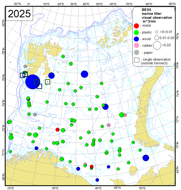
Surface observations of litter were carried out along the known-length transects of observations from marine mammal observers from Norwegian and Russian vessels. Some observations were made between the transects, so these data were not used in calculations.
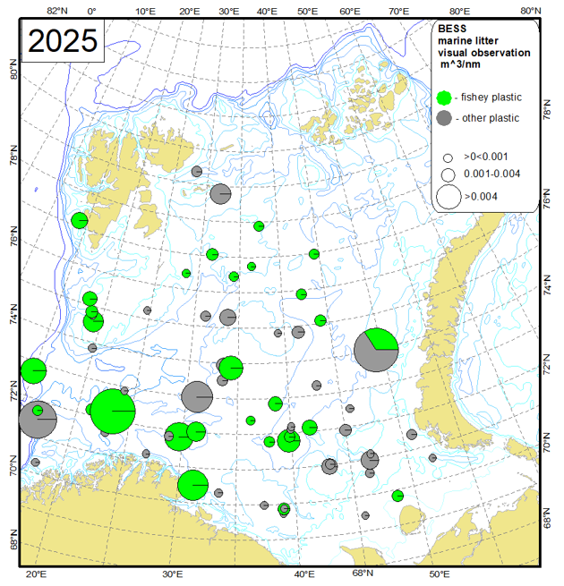
Plastic was the most frequent material type of floating litter observations (77.1 % of observations) (Fig. 4.2.1.1). The maximum surface observation of plastic litter was 0.005 m3 per nautical mile (m3/nm), and the average was 0.001 m3/nm. Fishery related litter was recorded in 43.2 % of plastic litter observations at the surface (Fig. 4.2.1.2). Fishery related plastic was represented by ropes, pieces of nets and floats/buoys. Fishery plastic maximum and average volume was 0.005 m3/nm and 0.001 m3/nm, respectively, and it is larger than non-fishery plastic (maximum and average observations of 0.004 m3/nm and 0.0005 m3/nm, respectively).
Wood (wooden sticks, pallets and logs) was recorded in 15.6 % of the surface litter observations. The maximum observation of wood was 0.03 m3/nm, with the average of 0.006 m3/nm. It should be noted that wood is the natural type of litter and biodegrades naturally in the environment.
Metal, paper and rubber were observed singularly (2.1-3.1 % of the observations).
Figure 4.2.1.1. Type of observed anthropogenic litter at the surface in the Barents Sea
in August-October 2025 (m3/nm).
Figure 4.2.1.2. Litter observations of plastic at the surface indicated as fishery related and other litter in the Barents Sea in August-October 2025 (m3/nm).
Observations of litter from the trawl transects were done during the survey. Onboard the Norwegian vessels litter from trawls were recorded according the ICES manual for seafloor litter data collection and reporting from demersal trawl samples (ICES Techniques in Marine Environmental Sciences. November 2022. Vol. 67). Onboard the Russian vessels a detailed description of the litter was carried out.
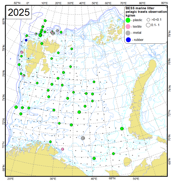
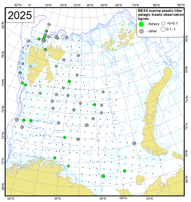
Anthropogenic litter was observed in 17.4 % of pelagic trawl stations during the survey (Fig. 4.2.1.3). Plastic usually is the most frequent material type observed in pelagic trawls and constituted 92.6 % of the observations (it was recorded in 16.1 % of all pelagic trawls). Weight of plastic litter from pelagic trawls varied from 0.0001 kg per nautical mile (kg/nm) to 0.022 kg/nm, with an average of all plastic observations of 0.003 kg/nm, and of all pelagic trawl stations of 0.0005 kg/nm. Fishery related litter (such as ropes made from synthetic fibres and pieces of fishing net) constituted 40.0 % of litter registrations from pelagic trawls (Fig. 4.2.1.4).
Other types of litter in pelagic trawls were metal (observed in 1.6 % of pelagic trawl stations and constituted 9.3 % of the litter observations), textile (in 1.3 % and in 7.4 % correspondingly) and rubber (was found only in one pelagic station). Weight of textile varied from 0.001 kg/nm to 0.005 kg/nm, weight of metal from 0.01 kg/nm to 0.02 kg/nm. It should be noted that textile is a natural product, e.g. ropes made from natural fibres (such as cotton, sisal, hemp, or coir) or all types of clothing (textile and woven products).
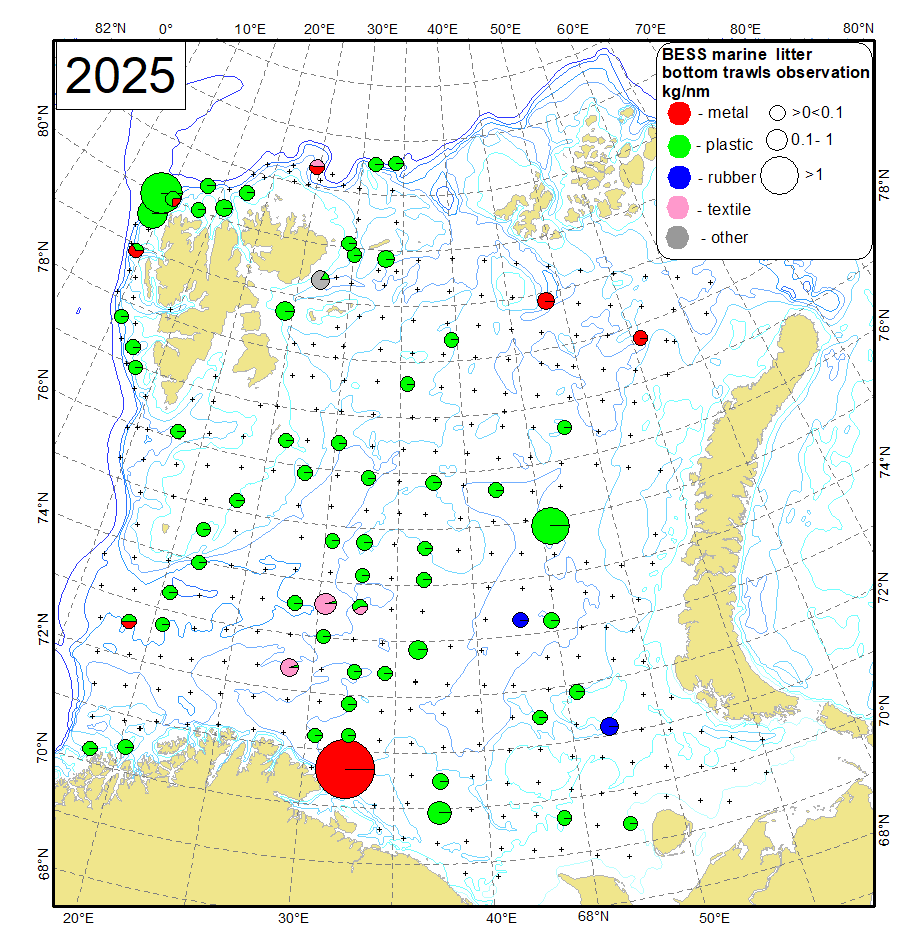
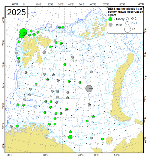
From the bottom trawls, 18.6 % of the stations contained litter (Fig. 4.2.1.5). Plastic was the most frequently observed material in the bottom trawls as in the pelagic (90.9 % of stations with observed litter and 16.9 % of the bottom trawls). Weight of plastic litter in bottom trawls varied from 0.0004 kg/nm to 0.766 kg/nm, with an average of 0.049 kg/nm in all bottom trawl stations, and of 0.008 kg/nm in bottom trawls with plastic registrations. Fishery related litter constituted 68.3 % of registrations from bottom trawls (Fig. 4.2.1.6).
Metal was found in 2.0 % of bottom trawl stations (in 10.6 % bottom trawls with litter registrations), weight of metal was from 0.001 kg/nm to 1.25 kg/nm. Textile belong to categories of natural product. It was observed in 1.1 % of bottom trawl stations (in 6.1 % bottom trawls with litter registrations). Weight of textile in bottom trawls varied from 0.006 kg/nm to 0.178 kg/nm. Other material types of litter observed in bottom trawls are rubber (was found at 2 stations) and unrecognisable items (at 1 station). It should be noticed that wood was not registered in bottom trawls during the survey in 2025, and this is the first time without such recordings during marine litter observations in the Barents Sea since 2010.
Figure 4.2.1.3. Type of anthropogenic litter collected in the pelagic trawls (kg/nm) in the Barents Sea in August-October 2025 (crosses – pelagic trawl stations).
Figure 4.2.1.4. Fishery related plastic observation versus other plastic litter collected in the pelagic trawls in the Barents Sea in August-October 2025 (kg/nm, crosses – trawl stations).
Figure 4.2.1.5. Type of anthropogenic litter collected in the bottom trawls (kg/nm) in the Barents Sea in August-October 2025 (crosses – bottom trawl stations).
Figure 4.2.1.6. Fishery related plastic observation versus other plastic litter collected in the bottom trawls in the Barents Sea in August-October 2025 (kg/nm, crosses – trawl stations).
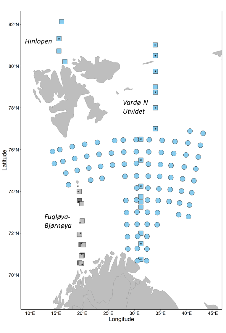
Samples used to characterize phytoplankton community composition and abundance were collected from a total of 116 stations over the course of three separate cruises. Microscopy and algae-net samples were collected from Hinlopen and Vardø-Nord Utvidet transects in October during the ecosystem cruise (cruise numbers: 2025102001, 2025002010), and Fugløya-Bjørnøya during Spring transect cruises conducted in April (cruise number: 2025002004) and June (cruise number: 2025002006). Microscopy was used to identify and quantify taxa in 32 preselected stations along the transects (Fig. 5.1.1). Algae-net samples, used to qualitatively evaluate community composition, were collected from 22 stations. In addition to the samples collected on fixed transects, samples for metabarcoding were collected from 81 stations in September from planned ecosystem cruise stations (cruise number: 2025001013). A subset of metabarcoding samples will be sequenced and analyzed as a part of a three-year time series characterizing phytoplankton community composition in the Barents Sea.
Samples for algal cell counts (100 ml) were taken from 10 m CTD collected water and fixed in Neutral Lugol. Microscope counts were performed following the Utermöhl (1958) method on CTD samples to quantify abundance and community composition at the IMR Flødevigen Plankton Laboratory. Qualitative Algae-net samples were collected using a vertical net tow (10 μm mesh; 0.1 m2 opening; 30-0 m), fixed with 2 ml 20% formalin in a 100 ml bottle and stored for future use. Metabarcoding samples were collected by filtering approximately 2 L of seawater, pre-filtered with 180 µm mesh, on to 25 mm filters with a pore size of 5 µm. Samples were then stored at -80 °C until DNA extraction and subsequent sequencing.
Microscopy algal counts include heterotrophic, mixotrophic, and autotrophic taxa, these communities will therefore be referred to as microplankton in the summarized results below.
5.1.2 Results
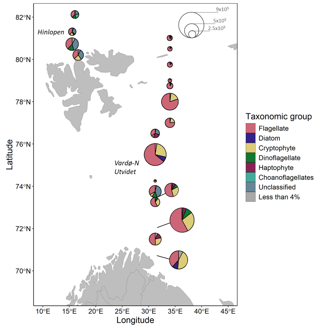
Based on microscopy counts, the average concentration of Barents Sea microplankton in October was 3.77×10⁵ ± 2.13×10⁵ cells L-1. The average community was numerically dominated by flagellates (56%, 2.13×10⁵ ± 1.32×10⁵ cells L-1) and cryptophytes (20%, 7.47×10⁴ ± 8.66×10⁴ cells L-1).
Microplankton abundances and communities varied spatially across the Barents Sea in October (Fig. 5.1.2). Cell concentrations varied by an order of magnitude between stations with a minimum concentration of 9.05×10⁴ cells L-1 and maximum of 8.67×10⁵ cells L-1. Higher concentration stations were generally found on the southern section of the Vardø-N Utvidet transect. In contrast to other stations, unclassified cells comprised large proportion of the Hinlopen station communities, these are likely flagellates whose flagella have fallen off.
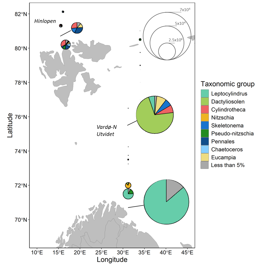
Within these data diatoms are the only purely photosynthetic group described at a high taxonomic level. In October diatom abundances were relatively low (<1×10⁵ cells L-1), with the most abundant stations found on the southern section of the Vardø-N Utvidet transect and Hinlopen stations nearest to the Svalbard/Spitsbergen coast (Fig. 5.1.3). Leptocylindrus and Dactyliosolen dominated the high abundance stations on Vardø-N. In contrast, the higher abundance stations on Hinlopen were split across multiple genera including Cylindrotheca, Pennales, Skeletonema, and Eucampia.
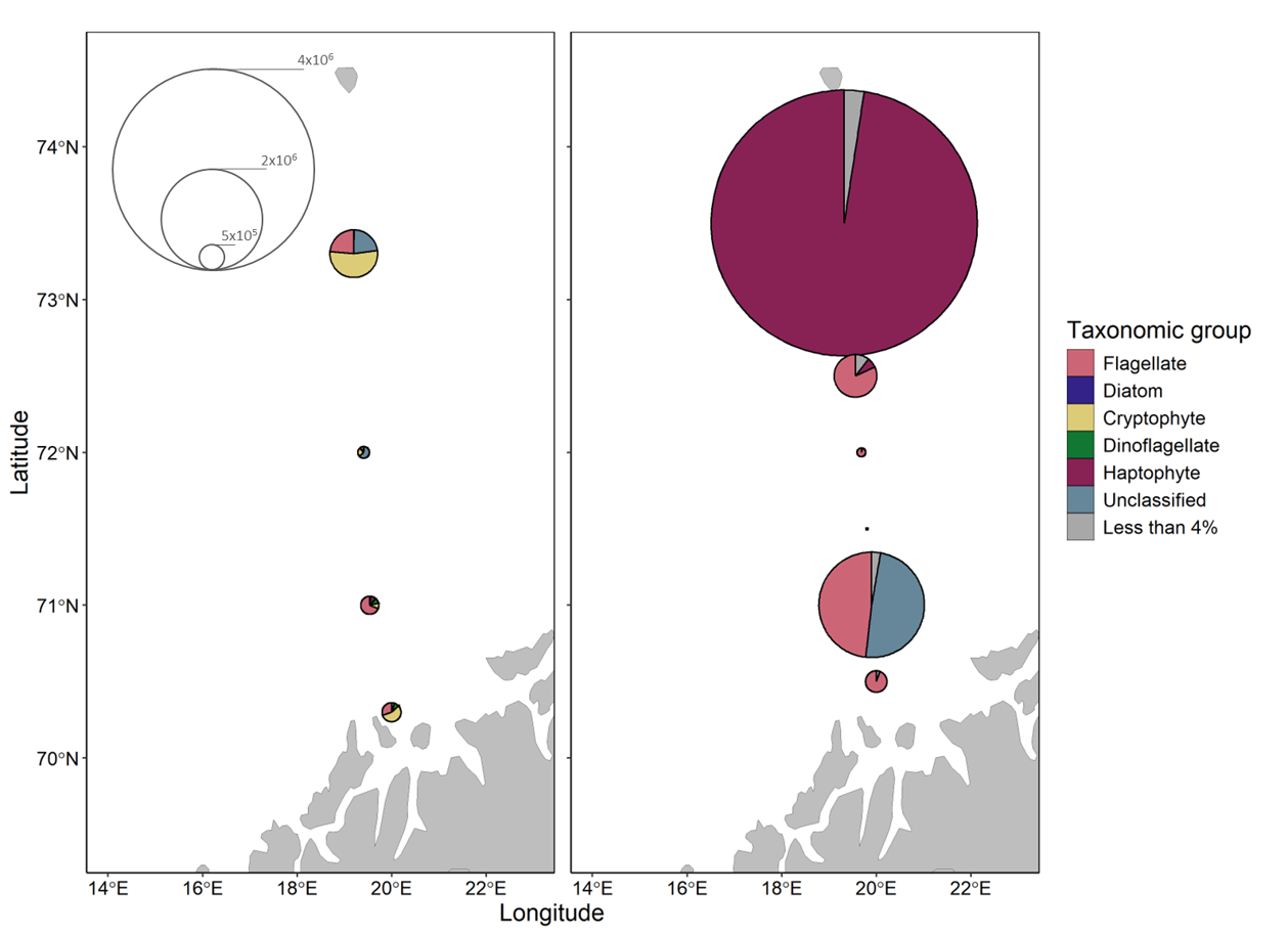
The combination of early (April) and late (June) spring sampling along the Fugløya-Bjørnøya transect allows us to describe the evolution of the spring bloom microplankton cell concentrations and community composition. Cell concentrations increased during the course of the spring with average cell concentrations of 3.89×10⁵ ± 3.41×10⁵ cells L-1 in April and 1.31×10⁶ ± 1.88×10⁶ cells L-1 in June, although June samples were characterized by greater intra-station variability (Fig. 5.1.4). At the broad taxonomic group level, April communities were dominated by flagellates and cryptophytes while haptophytes were more abundant in June. The high cell concentrations of haptophytes at the northernmost station in June document the occurrence of a Phaeocystis bloom, a common Spring bloom species in the Barents Sea.
Figure 5.1.1. Map showing stations where phytoplankton samples were collected. Shapes indicate sampling activities at a given station: circle- metabarcoding sample collection, square- microscopy sample collection and analysis, star: algae-net sample collection. Color indicates the cruise when sampling occurred, blue: ecosystem, dark gray: April transect cruise, light gray: June transect cruise. Italicized labels indicate fixed transects. Station locations along Fugløya-Bjørnøya are shifted to reduce overlap of samples collected during separate cruises.
Figure 5.1.2. Map showing microplankton community composition and abundance for samples collected during the 2025 Barents Sea Ecosystem cruise. Pie chart radii scale to cell concentrations in cells per liter based on key. Divisions within pie charts show the contributions from broad taxonomic groups. Italicized labels indicate fixed transects. All groups which comprised < 4% of the community are summed.
Figure 5.1.3. Map showing diatom community composition and abundance for samples collected during the 2025 Barents Sea Ecosystem cruise. Divisions within pie charts show taxonomic groups to the genus level. Pie chart radii scale to cell concentrations in cells per liter based on key. All groups which comprised < 5% of the community are summed.
Figure 5.1.4. Maps showing microplankton community composition and abundance for samples collected along the Fugløya-Bjørnøya transect in the Barents Sea. Samples were collected in April (left) and June (right). Divisions within pie charts show the contributions from broad taxonomic groups. Pie chart radii scale to cell concentrations in cells per liter based on key on the left. All groups which comprised < 4% of the community are summed.
5.2. Mesozooplankton biomass and geographic distribution
Text by: E. Bagøien and I. Prokopchuk
Figurs by: E. Bagøien
Mesozooplankton sampling stations during the joint Norwegian-Russian Barents Sea ecosystem cruise in 2025 are shown in Fig. 5.2.1. In the Norwegian sampling area the WP2 net (opening area ~ 0.25 m2) was applied, while in the Russian sampling area the Juday net (opening area ~ 0.11 m2) was used. Both gears were rigged with nets of mesh-size 180 mm and hauled vertically from near the bottom to the surface. The WP2 and Juday nets provide roughly comparable results with respect to mesozooplankton biomass and species composition (Skjoldal et al., 2019). The Norwegian biomass samples are dried before weighing, while the Russian samples are preserved in 4% formalin and their wet weight determined. Dry-weight is then estimated by dividing the wet-weight by a factor of 5.
The spatial distribution of total mesozooplankton biomass shown in Figure 5.2.1 is based on a total of 307 stations, of which 173 were sampled by the Norwegian vessels and 134 by the Russian vessel. Within the western part of the Barents Sea as represented by the Norwegian WP2 samples, the average biomass was 6.9 (± 5.1 SD) g dry-weight m-2. The average zooplankton biomass for the samples within the eastern part of the Barents Sea as represented by the Russian Juday samples was 8.2 (± 5.3 SD) g dry-weight m-2. All stations shown in Fig. 5.2.1 are included in the 2025 biomass averages here presented. Note that 10 stations in the central Barents Sea were sampled both by IMR and PINRO (not shown). In these specific cases the IMR data were excluded from Fig. 5.2.1 as well as the calculations of biomass given above.
The time-periods for zooplankton sampling by the Russian (26. Aug – 13. Oct 2025) and Norwegian (28. Aug – 3. Oct 2025) vessels were similar. Comparison of average biomasses across years is vulnerable to differing area coverages. Challenges in covering the same area over a series of years are inherent in such large-scale monitoring programs, and interannual variation in ice-cover and logistical issues are two of several reasons for this. To improve the regularity of the sampling grid of the survey area in 2025, stations along the Hinlopen Strait section located between Svalbard/Spitsbergen and Nordaustlandet (Svalbard/Spitsbergen) as well as the Vardø-North section that crosses the central Barents Sea, were excluded from Fig. 5.2.1 as well as the calculations of biomass averages. Differences in spatial coverage among years, as well as spatial variability in station density within the survey region will impact biomass estimates, and particularly so in an environment characterized by large-scale patterns in biomass distribution. Hence, the average biomasses for the Norwegian and Russian main areas as presented here are not directly comparable with those from earlier years.
Figure 5.2.1. Distribution of total zooplankton biomass (g dry-weight m-2) from near-bottom to surface in the Barents Sea during BESS 2025 – based on a total of 307 stations. The data visualized were collected by WP2 and Juday nets with mesh-size 180 mm. Interpolation was made in ArcGIS v.10.8, module Spatial Analyst, using inverse distance weighting (IDW).
Such challenges fall outside the scope of this cruise-report, but are addressed in other fora, for instance by analysing time-series within spatially consistent sub-areas.
The overall distribution patterns show similarities across years, although some interannual variability is apparent. In 2025 we observed the familiar pattern of comparatively high biomasses in the southwestern region, and northeast and east of Svalbard/Spitsbergen, as well as the deeper parts of the southeastern region. The biomasses were very low in the central regions including the bank areas, and in the southeastern corner of the Barents Sea (Fig. 5.2.1).
Several factors may impact the levels of zooplankton biomass in the Barents Sea;
Advective supply of zooplankton from the Norwegian Sea
Local zooplankton production rates – which are linked to temperature, nutrient conditions and primary production rates
Predation from carnivorous zooplankters (jellyfish, krill, hyperiids, chaetognaths, etc.)
Predation from planktivorous fish including capelin, young herring, polar cod, juveniles of cod, saithe, haddock, and redfish
Predation from marine mammals and seabirds
5.3 Macrozooplankton
5.3.1. Distribution and biomass of euphausiids
Text by: E. Eriksen, A. Dolgov, D. Prozorkevich and T. Prokhorova
Figures by: S. Karlson
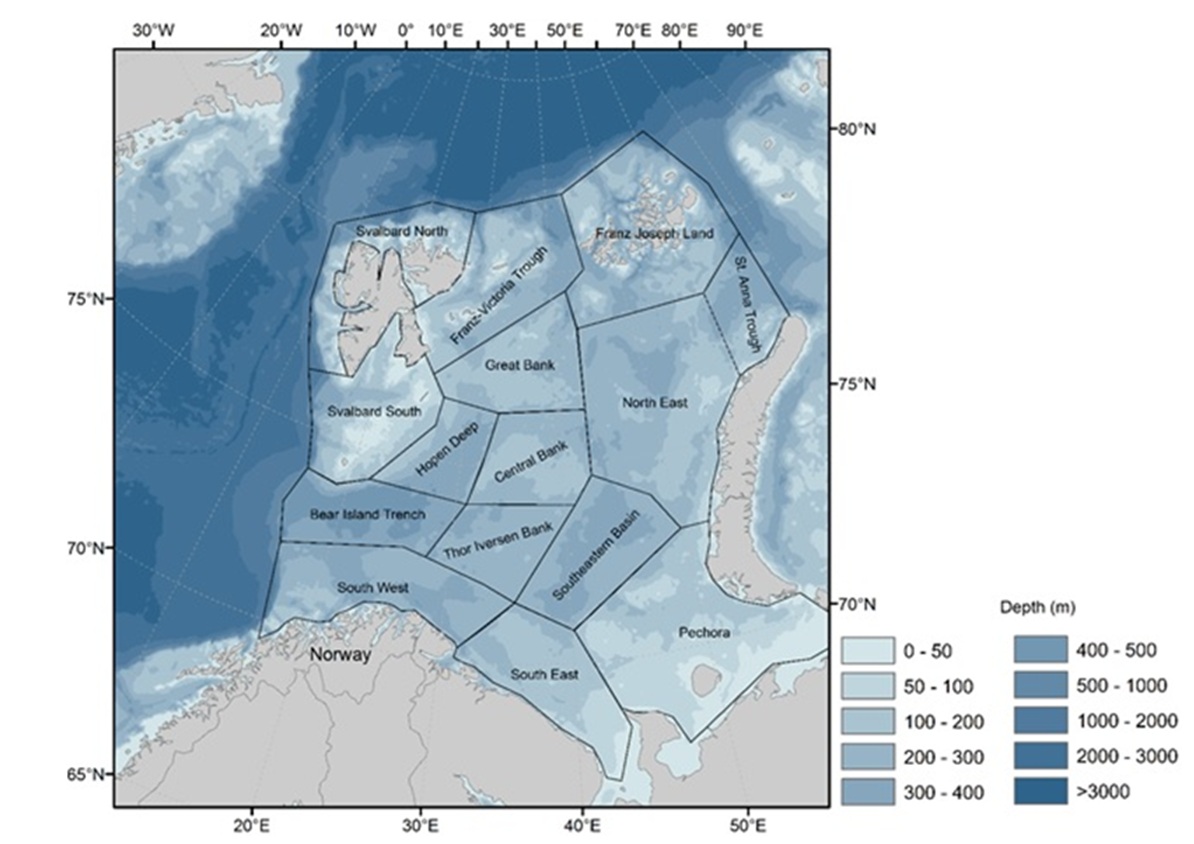
Biomass estimates were calculated by different software during the last four decades: Excel (up to 2017) and R (since that). The new 15 subareas, based on similar environmental status, were used since 2018 (Fig. 5.3.1), while two in the northeast seldom have observations. These areas were used to get more detailed information about the distribution of the krill within the survey area.
Figure 5.3.1. Map showing subdivision of the Barents Sea into 15 subareas (polygons) used to estimate macroplankton biomass based on the BESS.
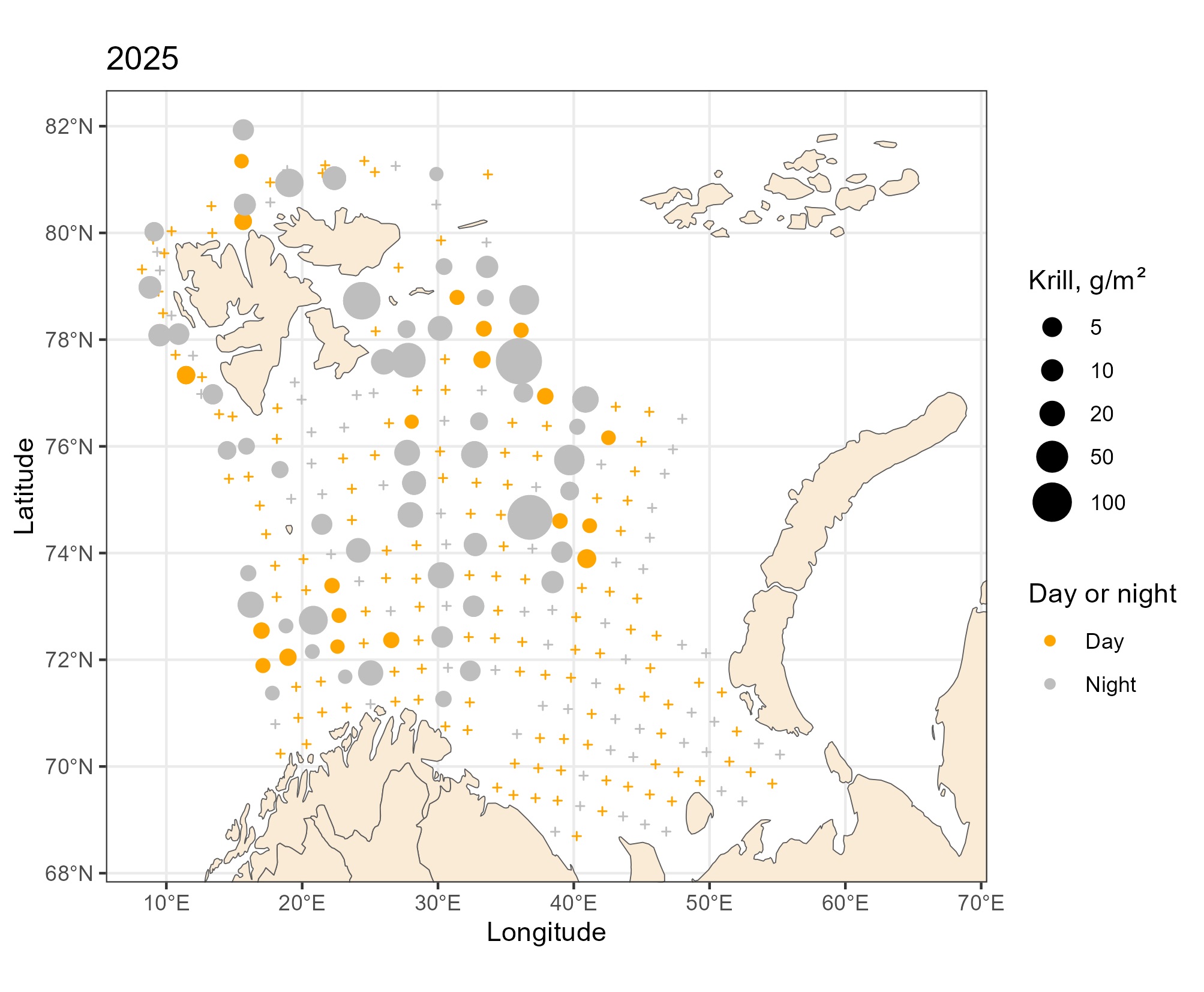
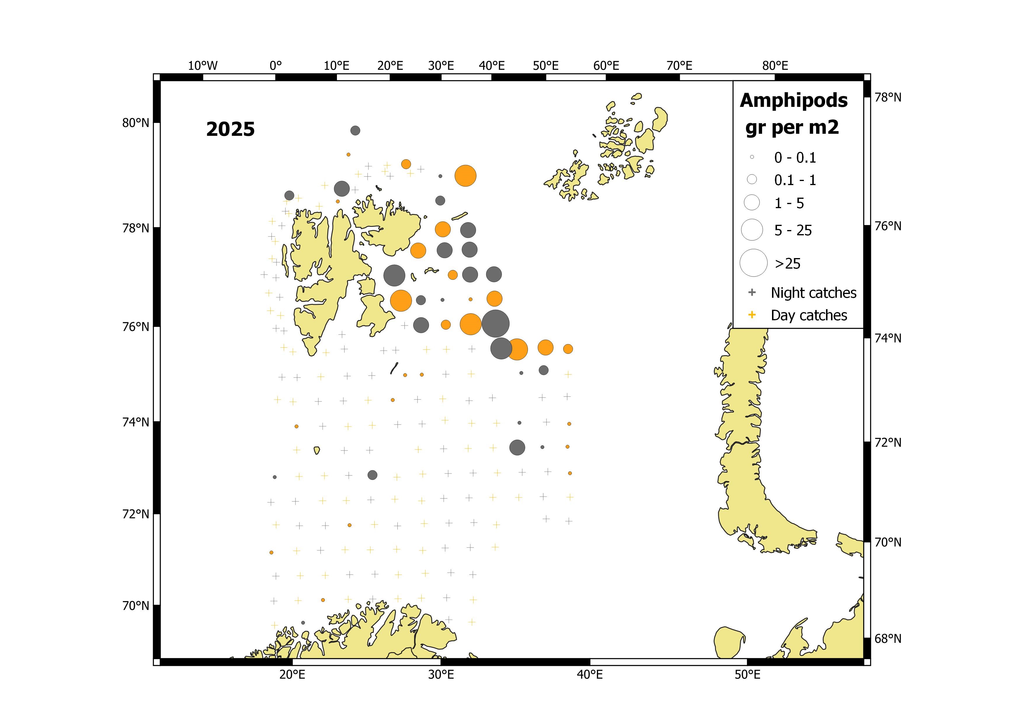
In 2025, euphausiids (krill) were widely distributed in the western and central Barents Sea with higher abundance in the southwest (Fig. 5.3.1.1). The biomass values in the upper 60 m are presented as grams (wet weight) per square meter (g/m2). In 2025, the night catches (mean 1.97 g/m2), were much lower than long term mean (7.3 g/m2).
Figure 5.3.1.1. Krill distribution (wet weight), based on pelagic trawl stations covering the upper water layer (0-60 m), in the Barents Sea in August-October 2025.
Figure 5.3.1.2. Krill distribution (species), based on pelagic trawl stations covering the upper water layer (0-60 m), in the Barents Sea in August-October 2025.
Based on the euphausiid species identification in 2025, Meganyctiphanes norvegica were widely observed in the Barents Sea, while Thysanoessa inermis were mainly observed in the central and northern areas. Two catches of Thysanoessa raschii were taken in the southwest and one in the Great Bank (Fig. 5.3.1.2). The smaller T. longicaudata were also found in 2025.
In 2025, the calculated total biomass of krill was 6.5 million tonnes which was lower that long term mean (fig. 5.3.1.3).
Figure 5.3.1.3. Estimated total biomass of krill in the Barents Sea in August-October 1980-2025 based on pelagic night trawl catches covering the upper water layer (0-60 m). Estimates in 1980-2001 were calculated based on average night catches of all night stations and total surveyed area. Estimates in 2003-2025 were calculated based on subarea average night catches and covered area within the subarea (Fig. 5.3.1). Estimates for 2002 are missing due to mistakes with the weight of krill.
Krill were captured at fewer number of trawl stations than in previous years, and especially east of Svalbard/Spitsbergen and in the southern Barents Sea, indicating possible high predation pressure from capelin and young herring respectively.
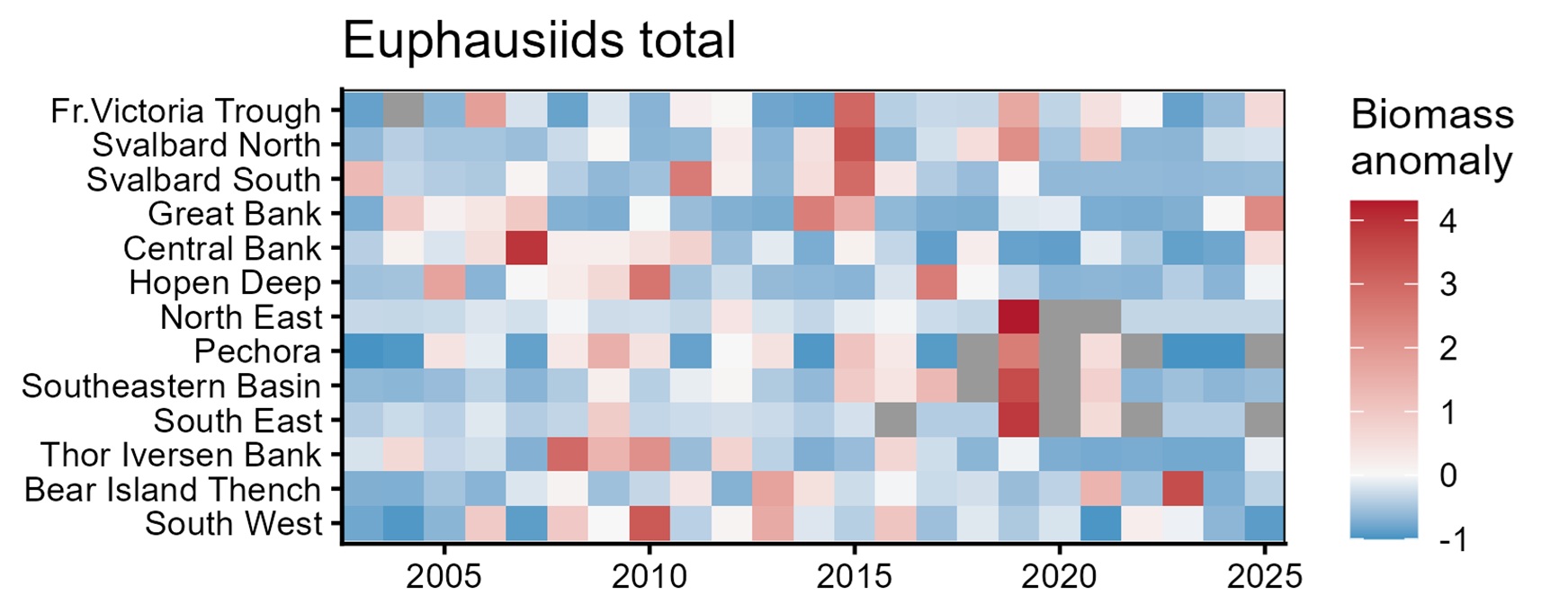
Spatial distribution of euphausiids biomass across 15 polygons in the Barents Sea (August–October, 2003–2025) are shown in Fig. 5.3.1.4.
Figure 5.3.1.4. Euphausiid biomass across 15 polygons in the Barents Sea (August–October, 2003–2025).
5.3.2 Distribution and biomass indices of pelagic amphipods (mainly Hyperiids)
Text by: E. Eriksen, A. Dolgov, D. Prozorkevich, T. Prokhorova and S. Karlson
Figures by: B. Husson and S. Karlson
Estimation of pelagic amphipods biomass for the Barents Sea was performed in R (see above) and presented here for the period 2003-2025.
In 2025, amphipods generally occurred east of Svalbard/Spitsbergen archipelago and few catches were also taken in the northern and central areas (Fig. 5.3.2.1).
Figure 5.3.2.1. Amphipods distribution, based on trawl stations covering the upper water layer (0-60 m), in the Barents Sea in August-October 2025.
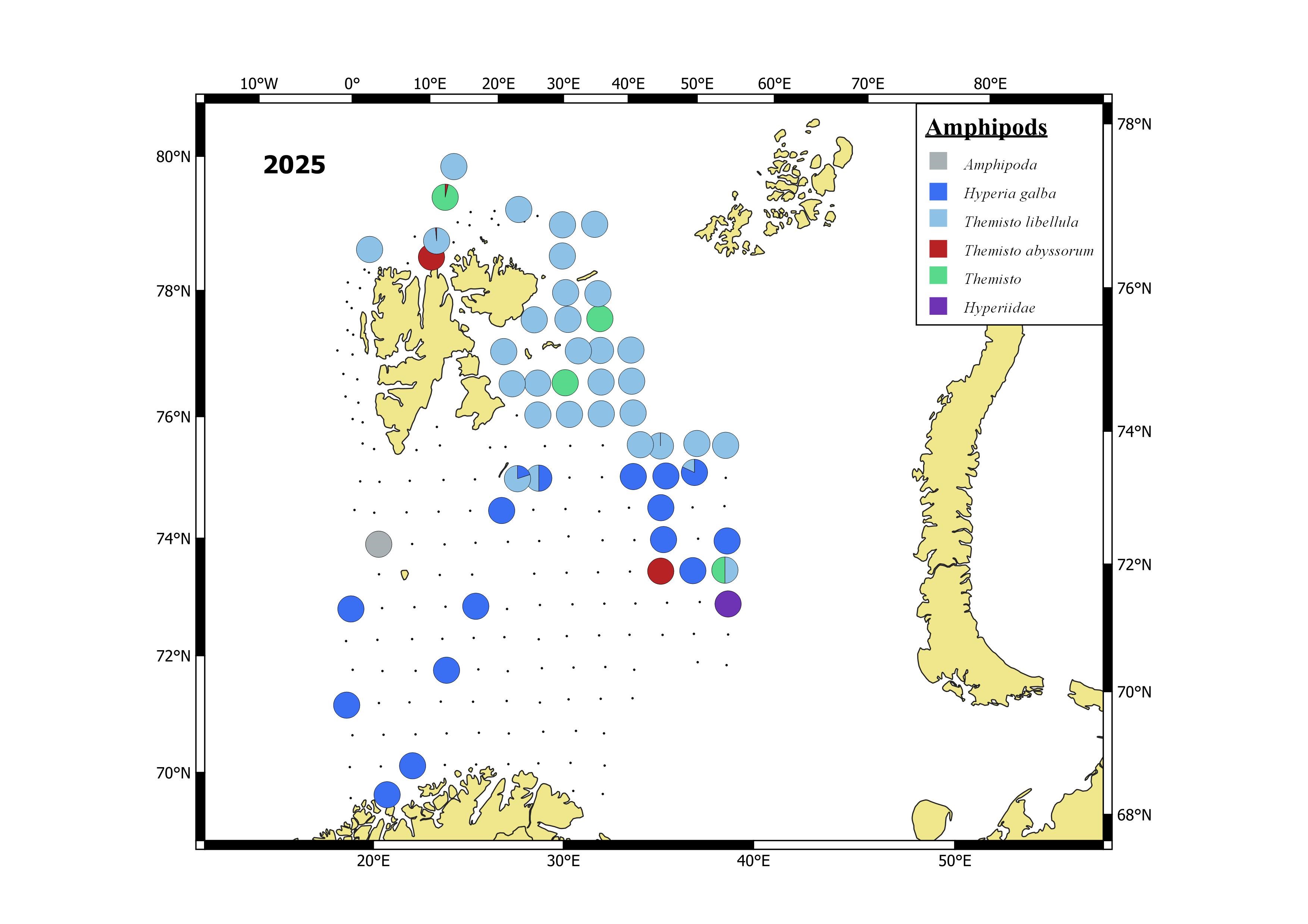
In 2025, amphipods taken Svalbard/Spitsbergen were mostly represented by the Arctic species Themisto libellula (Figure 5.3.2.2). The cosmopolitan species Hyperia galba were found in southwestern and north central areas. At two stations smaller Themisto abyssorum (with max measured length of 15.0 mm) were taken, while they are less captured by the trawl than larger T. libellula (with max measured length of 35.0 mm).
Figure 5.3.2.2. Distribution of pelagic amphipod species, based on pelagic trawl catches covering 0-60 m, in the Barents Sea in August-October 2025.
The calculated total biomass of amphipods in 2025 in the upper 60 m was 37.1 thousand tonnes, which is the lowest observed (Fig. 5.3.2.3).
Figure 5.3.2.3. Estimated total biomass of pelagic amphipods in the Barents Sea in August-October 2003- 2025, based on pelagic trawl catches covering the upper water layer (0-60 m). Estimates in 2003-2025 were calculated based on a subarea’s average catches and covered area within the subareas (Fig. 5.3.1.). In 2023, one catch makes a big difference in estimates: total biomass with this catch (red star) and without (blue line) are shown.
5.4. Distribution and biomass indices of jellyfish
Text by: E. Eriksen, S. Carlson, D. Prozorkevich, T. Prokhorova and A. Dolgov
Figures by: E. Eriksen and S. Carlson
The biomass of gelatinous zooplankton was calculated using SAS (for the new 23 fisheries subareas, 1980-2017). The new 15 subareas, based on environmental status and bathymetry, were used from 2018 to present spatial variation of jellyfish abundance and biomass (Fig. 5.4.1.). However, two polygons in the northeast seldom have observations.
R-script has been developed for three years, and during the last year some flaws in calculations were corrected. Thus, the biomass shown in previous reports may slightly differ from the latest one.
Here, we presented the time series for biomass indices calculated by SAS (1980-2017) and by R (2018-2025).
Figure 5.4.1. The new 13 subareas, based on environmental status and bathymetry, were used from 2018 to present spatial variation of jellyfish abundance and biomass.
The biomass of gelatinous zooplankton was calculated using SAS (for the new 23 fisheries subareas, 1980-2017). The new 13 subareas, based on environmental status and bathymetry, were used from 2018 to present spatial variation of jellyfish abundance and biomass (Fig. 5.4.2.). R-script has been developed for three years, and during the last year some mistakes in calculations were corrected. Thus, the biomass shown in previous reports may slightly differ from the latest one.
Here, we presented the time series for biomass indices calculated by SAS (1980-2017) and by R (2018-2025).
Figure 5.4.2. Distribution of jellyfish species (wet weight; kg per sq nmi) in the Barents Sea, August-October 2025.
The moon jellyfish (Aurelia aurita) was found at 39 stations in the southern Barents Sea with an average biomass of 14.6 tonnes per sq nmi (Fig. 5.4.2). This is the highest biomass of A. aurita ever observed.
Blue stinging jellyfish, Cyanea lamarckii, was found at 25 stations in the southwestern Barents Sea with average biomass 72.4 kg per sq nmi. C. lamarckii has been observed regularly in the Barents Sea in recent years and the presence of this warm-temperate species may be linked to the inflow of Atlantic water masses.
Ctenophores were found at 15 stations in the southern Barents Sea, and at six of these stations the ctenophores were also identified to genus level (Beroe spp.), commonly known as the cigar comb jellies. The average biomass was 60 kg per sq nmi and at five of these stations the calculated biomass was between 77 and 348 kg per sq nmi, that was also unusually high.
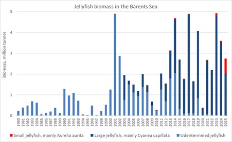
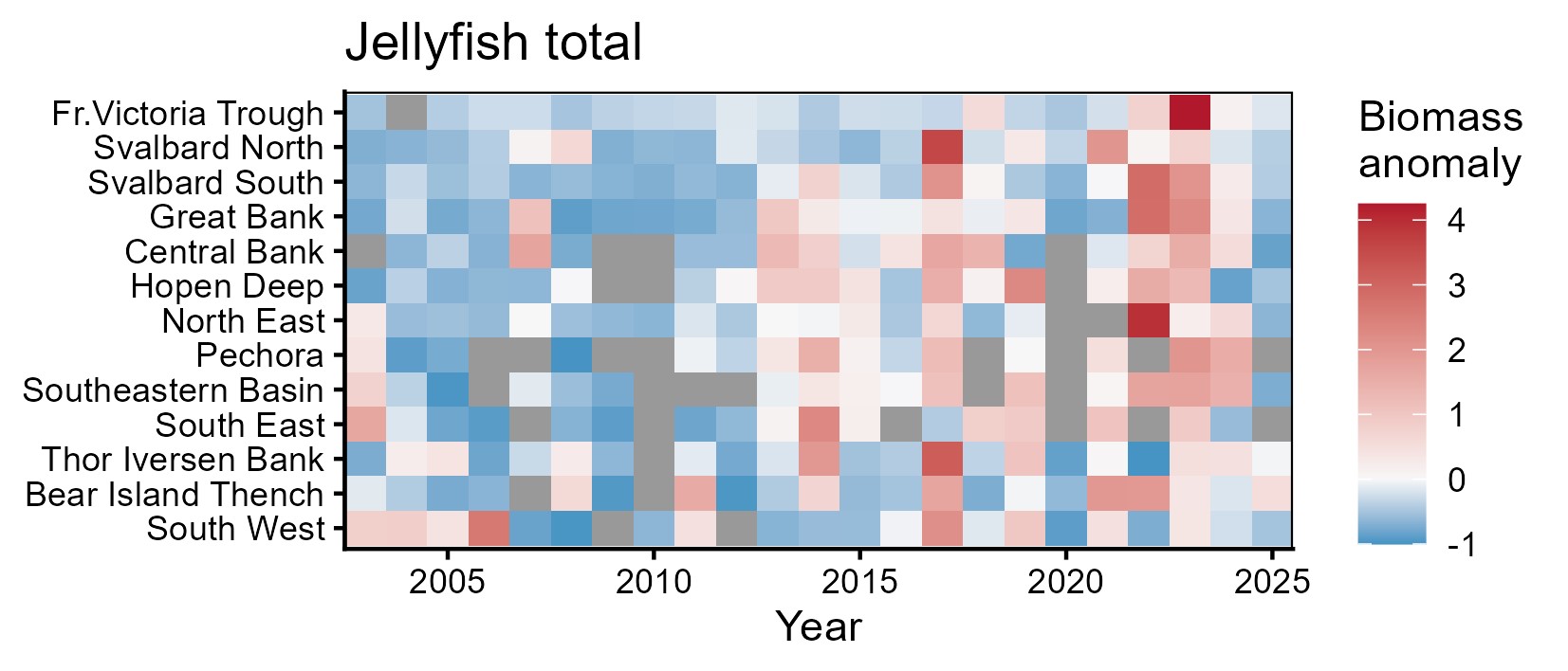
Biomass indices were calculated as total, for large jellyfish, dominating by C. capillata, small jellyfish dominating by A. aurita and unidentified jellyfish for the period 2004-2025. In 2025, total jellyfish biomass in the Barents Sea was much lower than in previously two years and was 2.746 million tonnes (Fig. 5.4.3). However, the proportion of small jellyfish increased from a few to 25% of the total jellyfish biomass index. Jellyfish biomasses dominated by biomasses of large jellyfish (2.0 million tonnes), although biomass of small jellyfish (dominated by Aurelia aurita) was the highest recorded (703 thousand tonnes, Fig. 5.4.3).
Figure 5.4.3. Total biomass of jellyfish in the Barents Sea in August-September 1980-2025. Large jellyfish were dominating by C. capillata, small jellyfish dominated by A. aurita, and other jellyfish (found occasionally). Biomass estimates in 2018, 2020 and 2022 were underestimated due to lack of coverage.
Geographical distribution of jellyfish, mainly C. capillata, showed decrease in all areas, except Bear Island Trench in 2025 (Fig. 5.4.4).
Figure 5.4.4. Geographical distribution of jellyfish, mainly C. capillata in 13 polygons in August-September 2003-2025.
In 2025, the overall coverage of the 0-group distribution was good, with the exception of the polar cod distribution areas in east and the northeastern parts of the Barents Sea (Fig. 6.1). This area has usually not been surveyed in recent years due to time constraints. The abundance and biomass of the zero-group fish were previously calculated using various software packages: SAS&MSAccsess (1980-2015), MatLab (2016-2019), and R (2019-2025). A re-estimation of the zero group time series from BESS using StoX is almost complete and will be presented in a separate report, with the aim to implement it as official estimate from next year.
Figure 6.1. Map showing spatial coverage of the 0-group sampling stations in the Barents Sea in 2025. The color of the dots indicate vessels, while the blue lines indicate 15 subareas (regions) used for the estimations.
6.1 Capelin (Mallotus villosus)
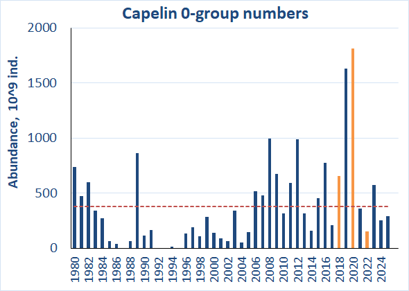
Capelin were distributed widely, but for the most part at low densities (Fig. 6.1.1), in accordance with an abundance estimate below average (Fig. 6.1.2). The distribution indicates that some capelin were outside the survey area in the north. The highest densities were observed in the central part and north of Svalbard/Spitsbergen.
Figure 6.1.1. Distribution of 0-group capelin, August-September 2025. Variations of blue color indicate fish densities, while the dots indicate sampling locations.
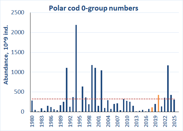
Figure 6.5.2. Estimated abundance of 0-group polar cod corrected for capture efficiency (Keff) for the period 1980-2025. Red dotted line shows the long-term average. Abundance indices for 2018, 2020 and 2022 were adjusted due to lack of survey coverage and are shown in orange colour.
6.2 Cod (Gadus morhua)
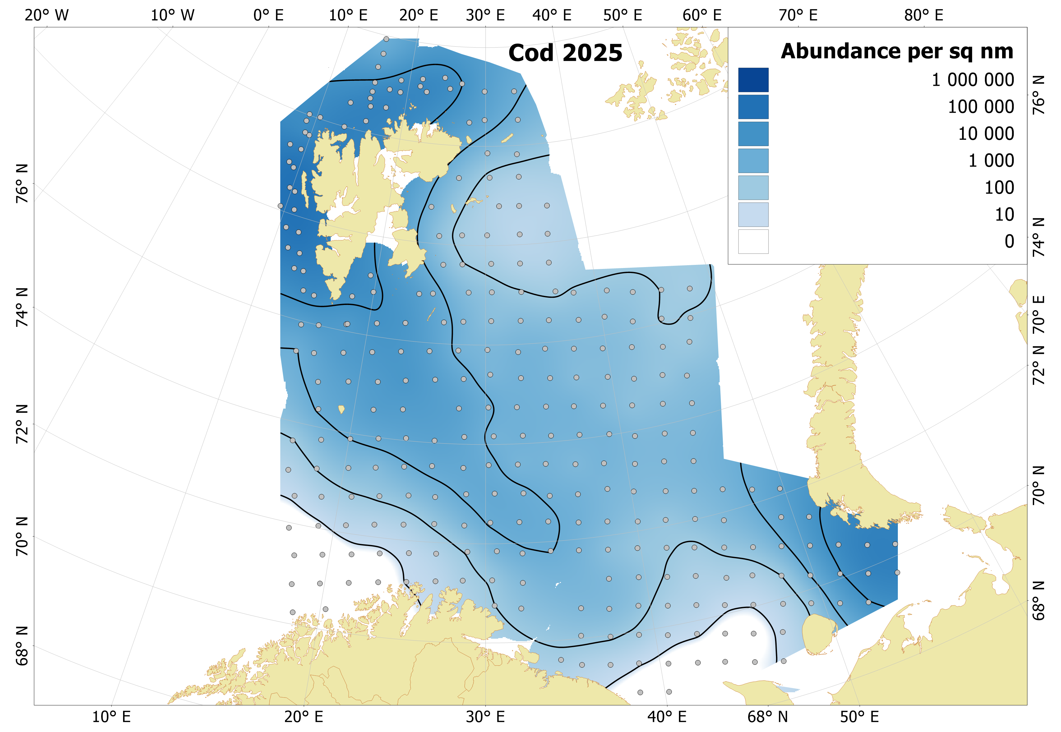
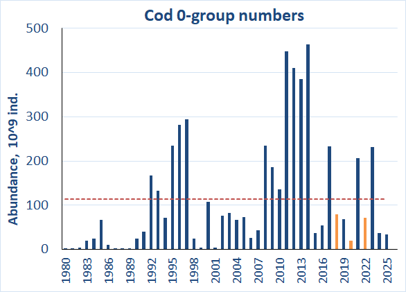
Cod were widely distributed in the Barents Sea but in low densities. The highest densities were found in the southeast and northwest parts of Barents Sea, and some fish were likely distributed outside the survey area (Fig. 6.2.1). In accordance with the low densities, the abundance estimate indicated a poor year class of cod in 2025 (Fig. 6.2.2).
Figure 6.2.1. Distribution of 0-group cod, August-September 2025. Variations of blue color indicate fish densities, while the dots indicate sampling locations.
Figure 6.2.2. 0-group cod abundance estimates corrected for capture efficiency (Keff) for the period 1980-2025. Red line shows the long-term average. Abundance indices for 2018, 2020 and 2022 were corrected for lack of coverage and shown by orange columns.
6.3. Haddock (Melanogrammus aeglefinus)
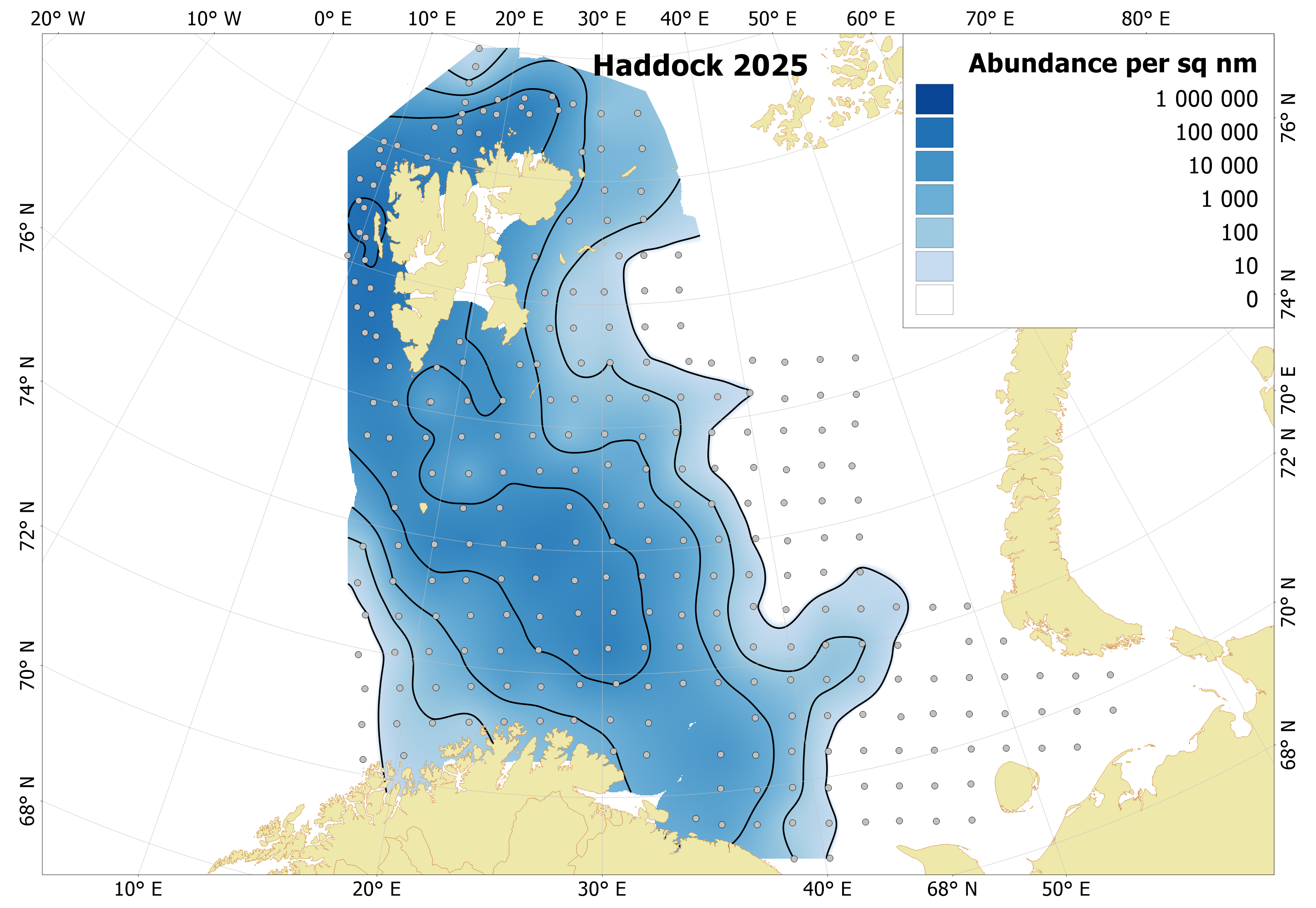
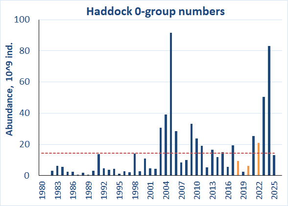
Haddock were distributed in the western and central parts of the Barents Sea, mainly west of 40°E (Fig. 6.3.1). High densities were not observed in the survey area. In accordance with low densities, the abundance estimate was low indicating a low 2025 year class (Fig. 6.3.2).
Figure 6.3.1. Distribution of 0-group haddock, August-September 2025. Variations of blue color indicate fish densities, while the dots indicate sampling locations.
Figure 6.3.2. 0-group haddock estimates corrected for capture efficiency (Keff) for the period 1980-2025. Red line shows the long-term average. Abundance indices for 2018, 2020 and 2022 were corrected for lack of coverage and shown by orange columns.
6.4 Herring (Clupea harengus)
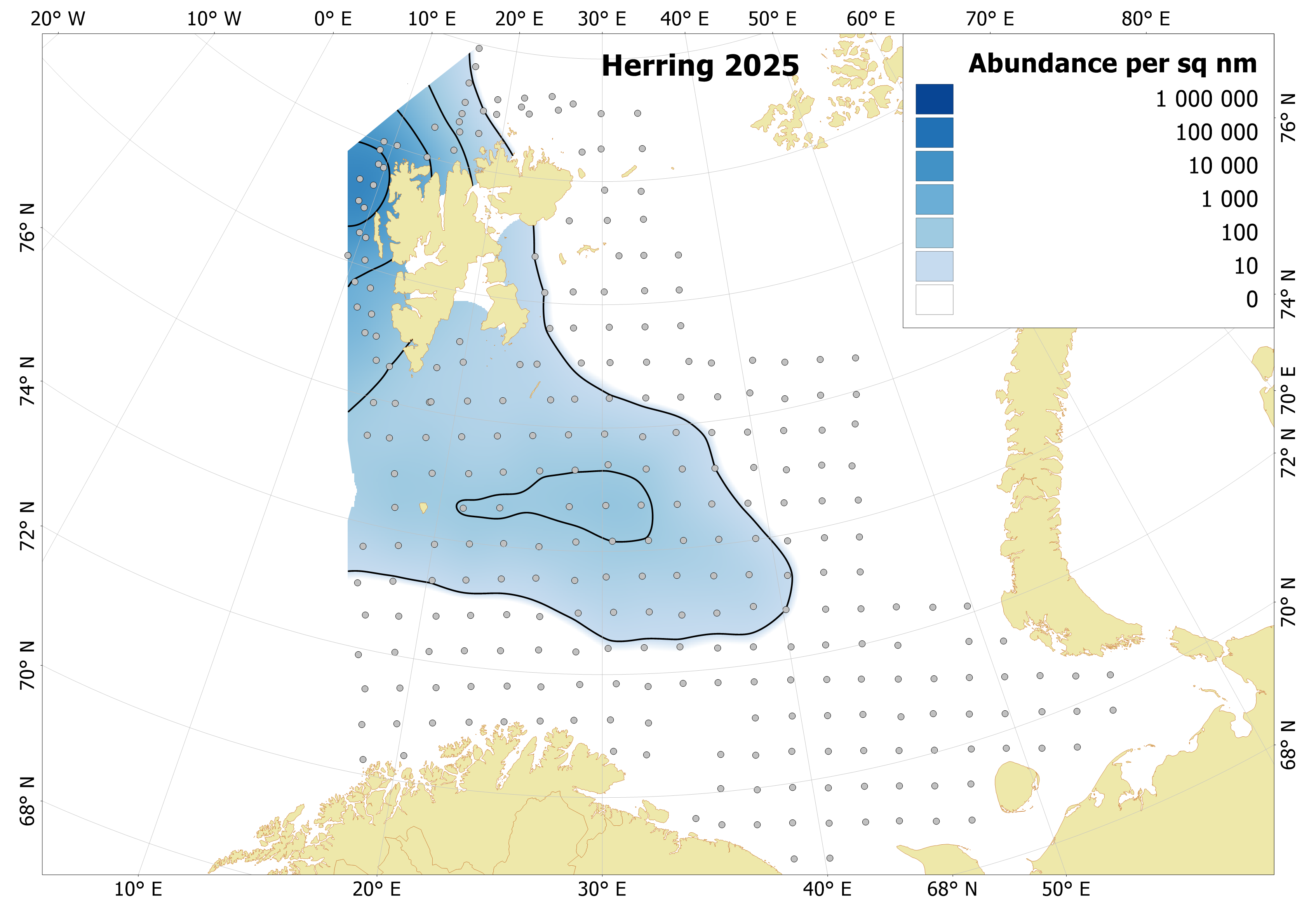
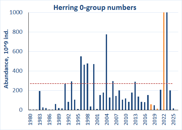
Distribution of herring was limited to a very small area (Fig. 6.4.1), with the highest densities northwest of Svalbard/Spitsbergen. The abundance in 2025 was extremely low, and far below the long term level (Fig. 6.4.2).
Figure 6.4.1. Distribution of 0-group herring, August-September 2025. Variatons of blue color indicate fish densities, while the dots indicate sampling locations.
Figure 6.4.2. Estimated abundance of 0-group herring corrected for capture efficiency (Keff) for the period 1980-2025. Red dotted line shows the long-term average. Abundance indices for 2018, 2020 and 2022 were adjusted due to lack of survey coverage and are shown in orange colour. For 2022 (2015*109 ind.) and 2023 (3624*109 ind.) the values are outside the graph axis.
6.5 Polar cod (Boreogadus saida)
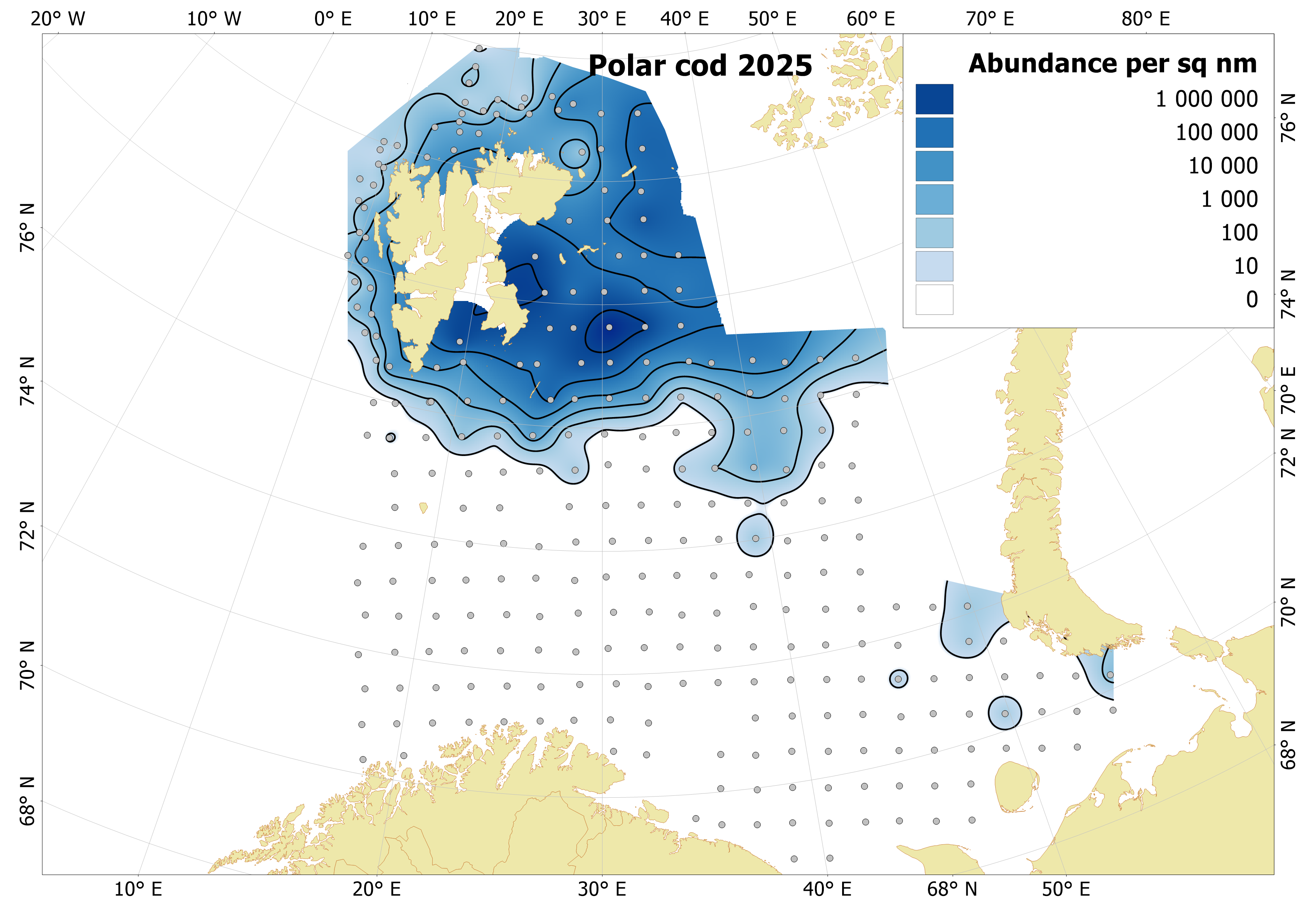
Polar cod were found around the Svalbard/Spitsbergen and in the eastern Barents Sea in 2025 (Fig. 6.5.1). There is an increasing shift northwards in the distribution of zero group polar cod. Coverage of the 0-group polar cod was not complete, and especially the eastern parts of the Barents Sea lacked coverage (Fig. 6.5.1). As a consequence, the south-eastern component of the polar cod is not fully represented here. The abundance estimate was slightly below the long term average, but given the lack of coverage in potentially important distribution areas, the true abundance is higher than estimated and year class strength is possibly strong in 2025 (Fig.6.5.2). It should be noted that estimates of the year class strength of polar cod is associated with high uncertainty.
Figure 6.5.1. Distribution of 0-group polar cod, August-September 2025. Variations of blue color indicate fish densities, while the dots indicate sampling locations.
Figure 6.5.2. Estimated abundance of 0-group polar cod corrected for capture efficiency (Keff) for the period 1980-2025. Red dotted line shows the long-term average. Abundance indices for 2018, 2020 and 2022 were adjusted due to lack of survey coverage and are shown in orange colour.
6.6. Saithe (Pollachius virens)
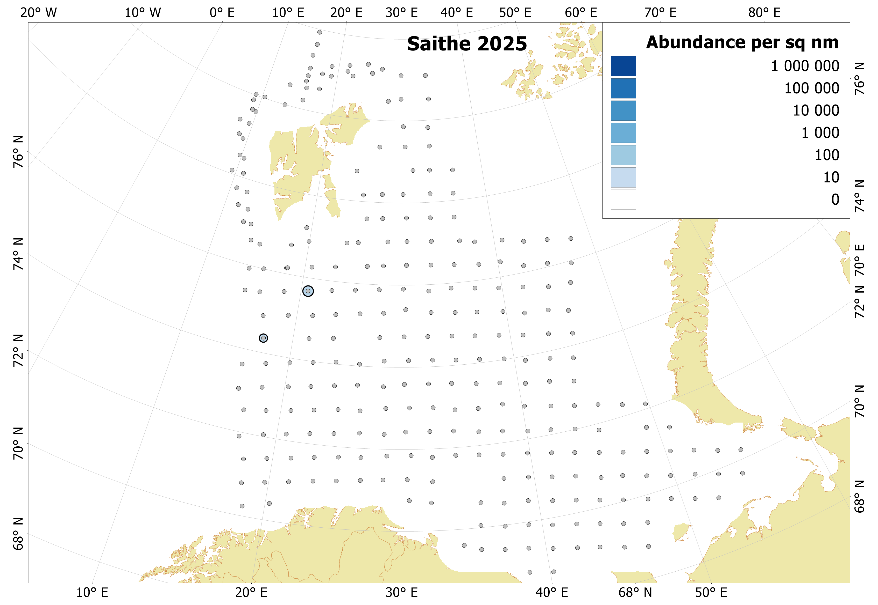
In 2025, there were hardly any 0-group saithe sampled, only a few specimens were caught (Fig. 6.6.1). This could be due to an abnormal saithe distribution (e.g. in coastal areas outside the survey coverage area) and/or a poor year class.
Figure 6.6.1. Distribution of 0-group saithe, August-September 2025. Variations of blue color indicate fish densities, while the dots indicate sampling locations.
6.7. Redfish (mostly Sebastes mentella)
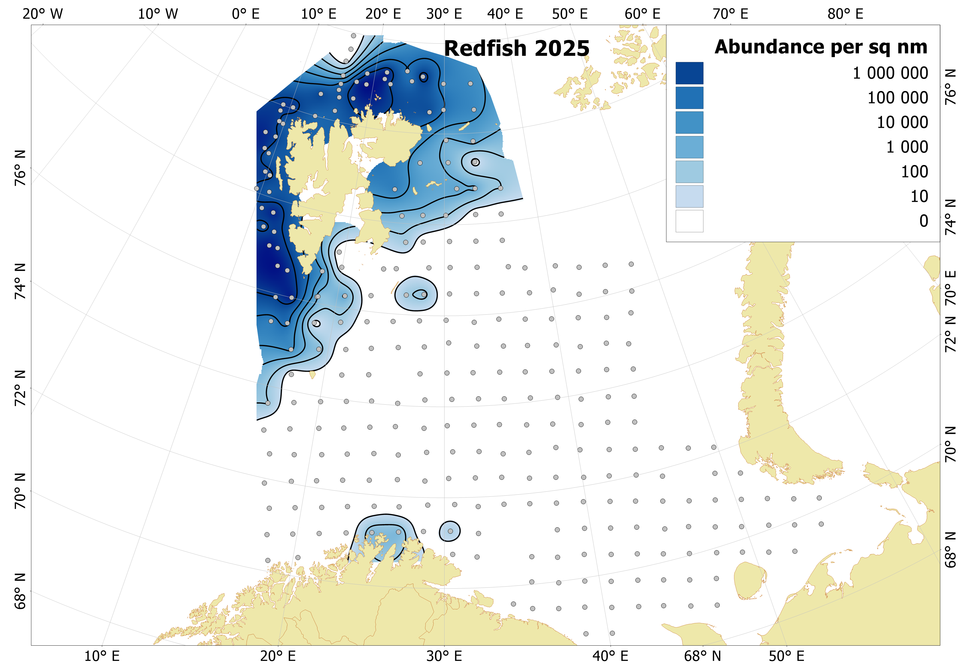
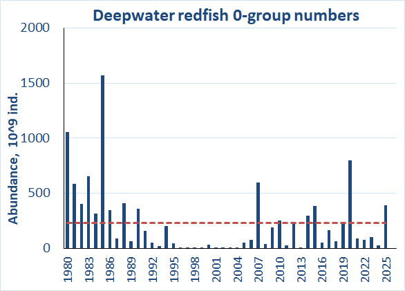
0-group redfish were found close to the north of the Norwegian coast and around Svalbard/ Spitsbergen in 2025. High densities were observed around Svalbard/Spitsbergen (Fig. 6.7.1). The 2025 abundance is the highest in 5 years and slightly above the long-term average (Fig. 6.7.2).
Figure 6.7.1. Distribution of 0-group redfish (mostly Sebastes mentella) in August-September 2025. Variations of blue color indicate fish densities, while the dots indicate sampling locations.
Figure 6.7.2. 0-group deepwater redfish abundance corrected for trawl efficiency (Keff) in the Barents Sea during 1980-2025. Red line shows the long-term average.
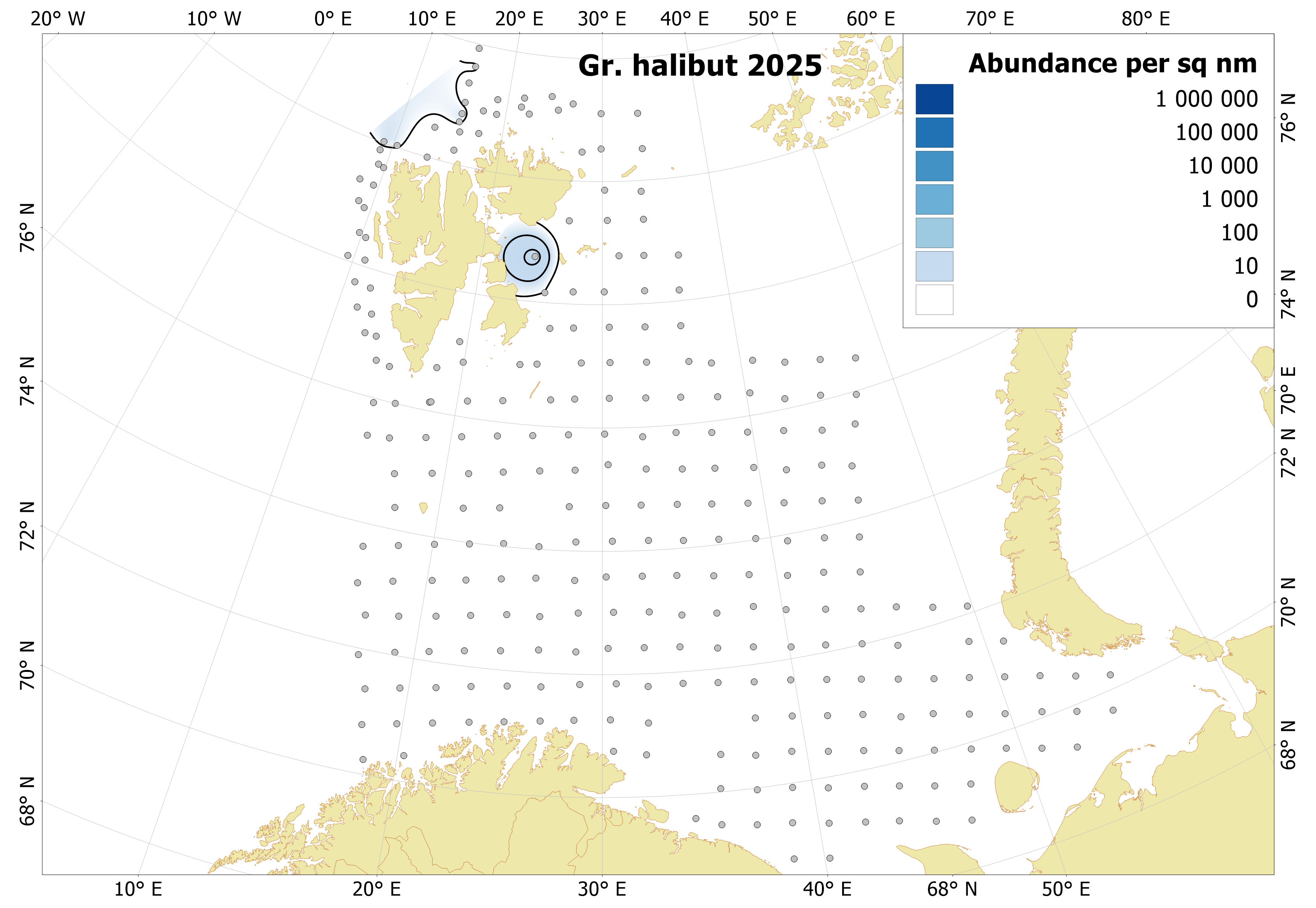
0-group Greenland halibut was found on several stations around of Svalbard/Spitsbergen in 2025 (Figure 6.8.1). Greenland halibut is typically distributed in the fjords of Svalbard/Spitsbergen or in deep depths in the open sea, but 0-group survey provide information about overall distribution, which reflects the abundance of year-classes, can be some signal for assessed. No successful generations of halibut have been recorded in recent years.
Figure 6.8.1. Distribution of 0-group Greenland halibut, August-September 2025. Variations of blue color indicate fish densities, while dots indicate sampling locations.
6.9. Long Rough dab (Hippoglossoides platessoides)
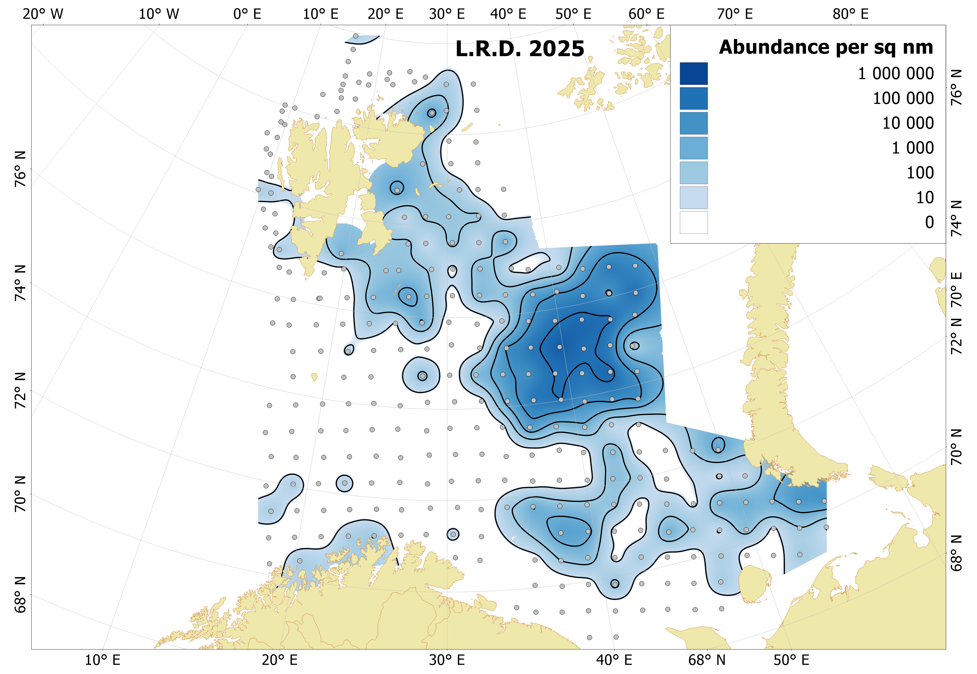
The 0-group of long rough dab (LRD) was widely distributed from northwest to southeast, with the highest densities observed in the central part of the Barents Sea.
No numbers estimate was made for 2025, but compared to previous years, the 2025 year-class appears to be very numerous and above long-term average level. Large numbers of 0-group LRD were also caught in bottom trawls catches supporting that they were numerous this year.
Figure 6.9.1. Distribution of 0-group long rough dab, August-September 2025. Variations of blue color indicate fish densities, while dots indicate sampling locations.
7 - Commercial Pelagic Fish
Author(s):
Georg Skaret
(IMR) and Dmitry Prozorkevich (VNIRO-PINRO)
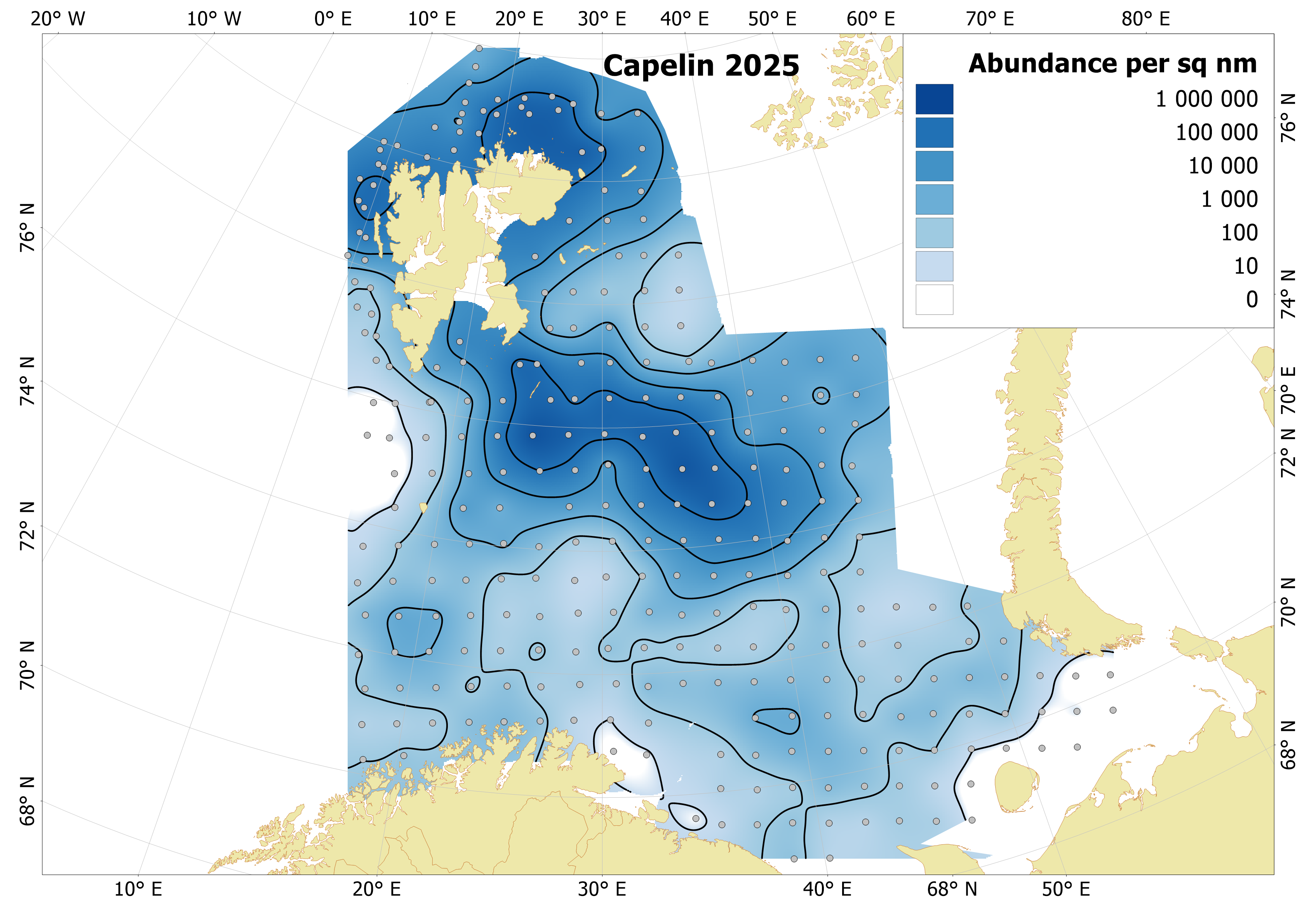
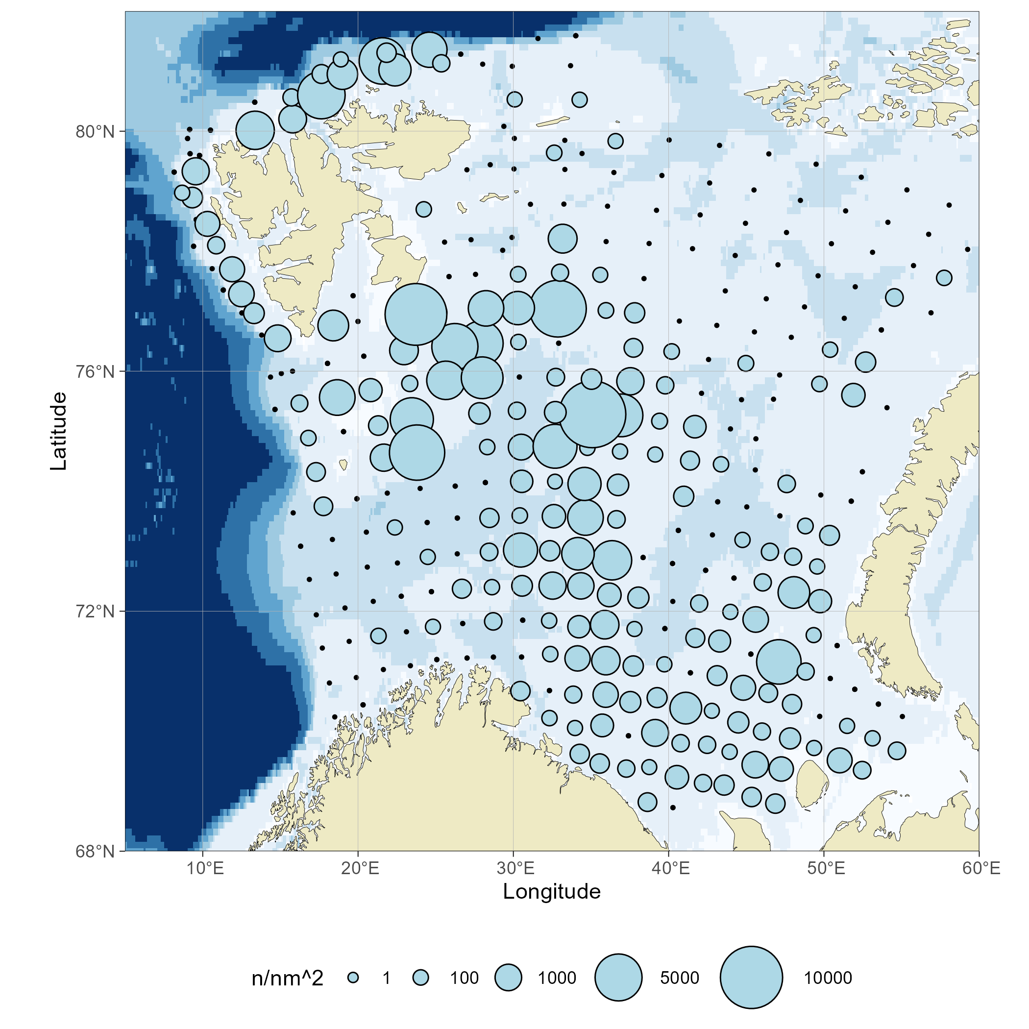
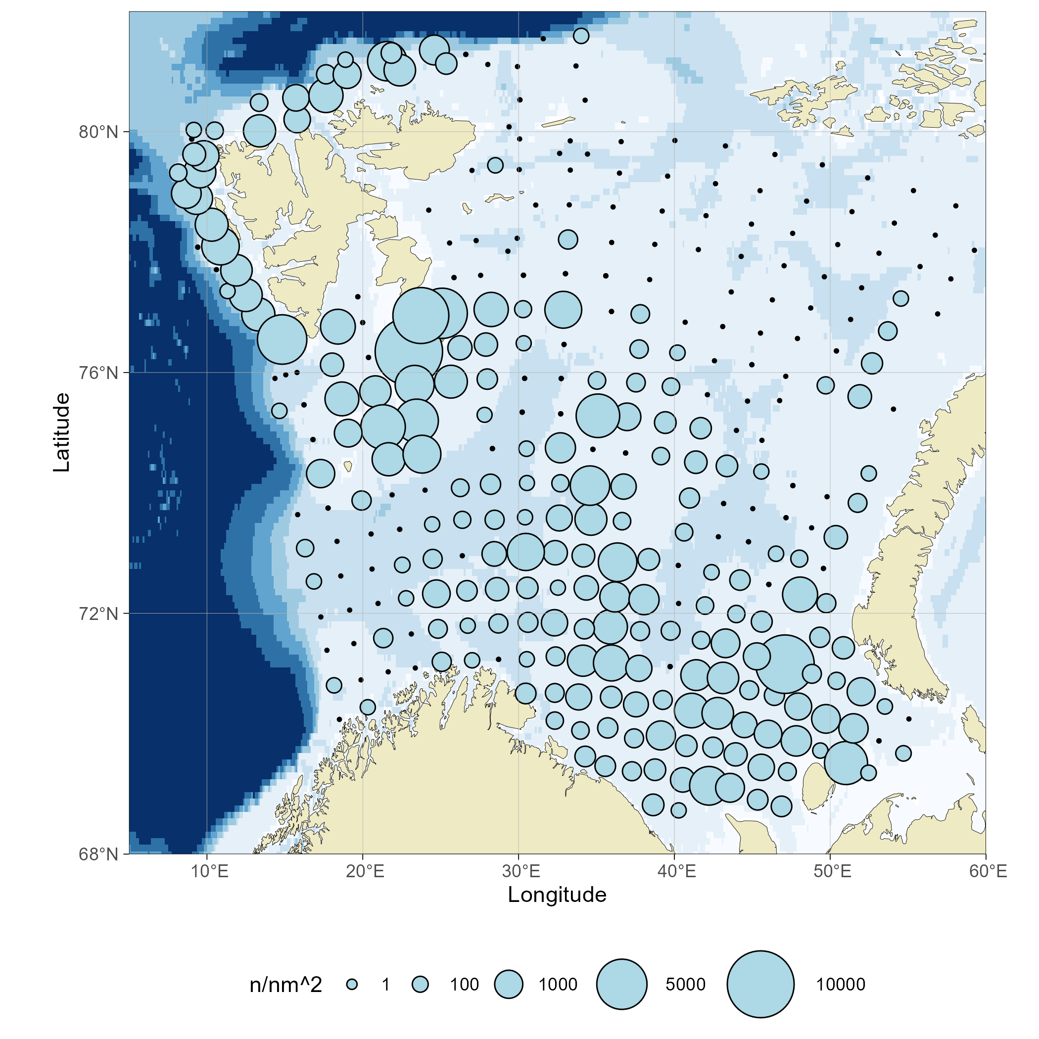
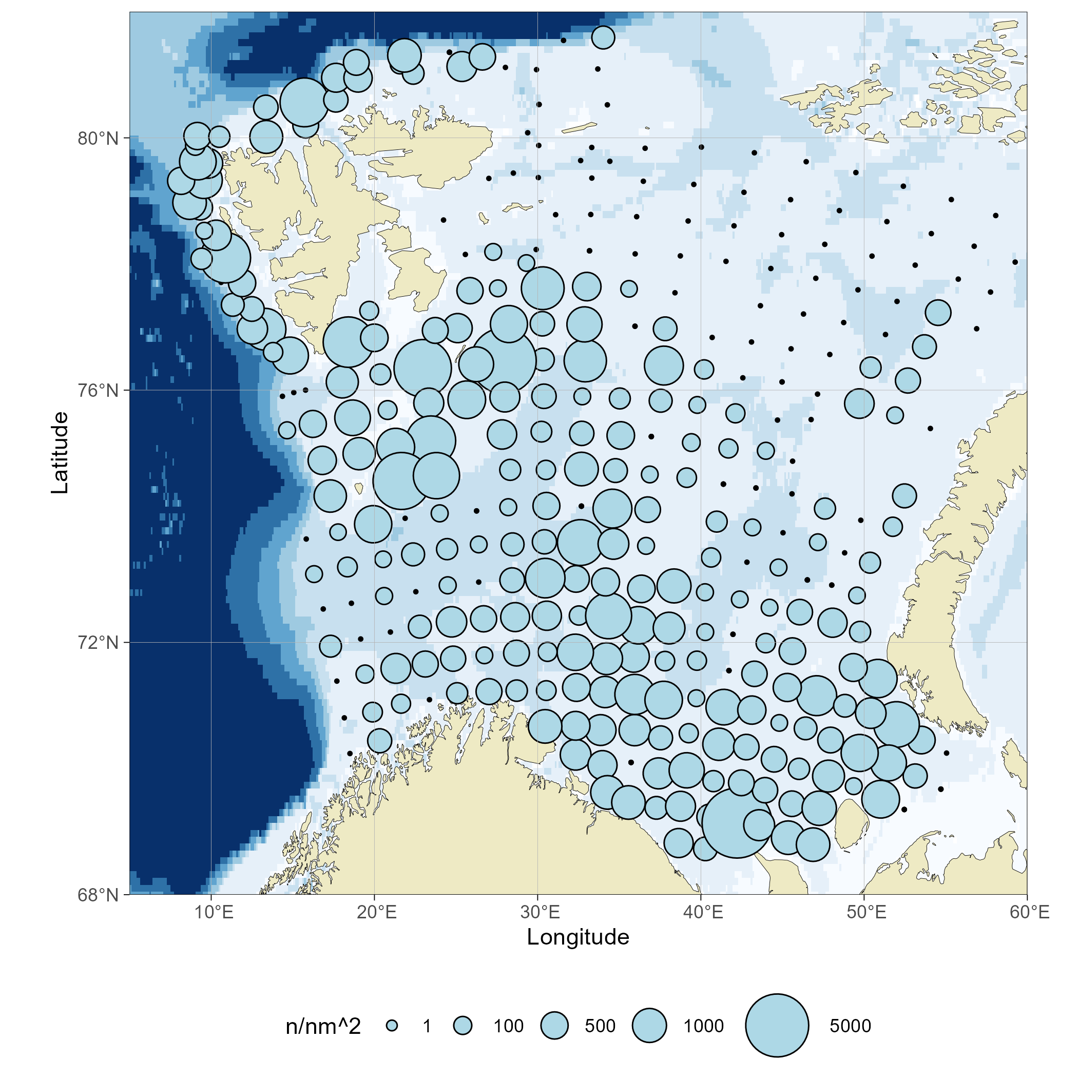
The geographical distribution of capelin recorded acoustically is shown in Fig. 7.1.1.1. The capelin was distributed further south than in 2024, and notably there were very small amounts of capelin in the Great Bank area and east of the Russian/Norwegian boundary. Significant capelin recordings north and west of Svalbard/Spitsbergen have been made in this survey in recent years and were made also this year.
Figure. 7.1.1.1. Geographical distribution of capelin in autumn 2025 based on acoustic recordings. Circle sizes correspond to NASC values (m2/nmi2) per nautical mile.
7.1.2 Abundance by size and age
A detailed summary of the acoustic stock estimate is given in Tab. 7.1.2.1, and the time series of abundance estimates is summarized in Tab. 7.1.2.2. A comparison between the estimates in 2025 and 2024 is given in tab. 7.1.2.3 with the 2024 estimate shown on a shaded background.
The total stock in the covered area was estimated to about 339 thousand tons, which is only about 13% of the long-term average level (2.71 million tons). About 37 % (124 thousand tons) of the 2025 stock had length above 14 cm and was therefore considered to be maturing. The contribution to the total in biomass and numbers was highest from 1 and 2-year-olds (table 7.1.2.1). The biomass of all year classes was less than the long-term average and for 2 and 3-year-olds, the biomass was 10% or less than the long-term average (table 7.1.2.2).
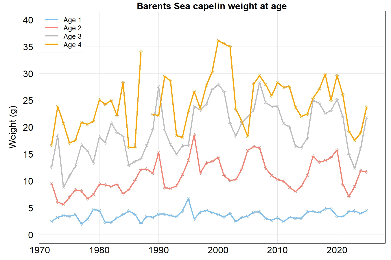
Average weight at age increased compared to 2024 for the age groups 1, 3 and 4. For 3- and 4-year-olds it was still well below the long-term average, whereas it was above the long-term average for 1 and 2-year-olds (fig. 7.1.2.1 and tab. 7.1.2.2).
Table 7.1.2.1. Barents Sea capelin. Summary of results from the acoustic estimate in August-September 2025. The table is generated from the mean of 1000 bootstrap replicates based on calculations in StoX 4.1.1. TSN denotes total stock number, TSB total stock biomass, SSN maturing stock number and SSB maturing stock biomass.
Length (cm)
Age/year class
Sum (109)
Biomass (103 t)
Mean weight (g)
1
2
3
4
5
2024
2023
2022
2021
2020
6.0-6.5
0.004
0.004
0.004
1.00
6.5-7.0
0.264
0.264
0.264
1.00
7.0-7.5
1.792
1.792
2.516
1.40
7.5-8.0
1.483
1.483
1.892
1.28
8.0-8.5
2.386
0.410
2.796
5.909
2.11
8.5-9.0
2.705
0.021
2.726
6.957
2.55
9.0-9.5
2.496
2.496
7.669
3.07
9.5-10.0
3.841
0.142
3.984
14.475
3.63
10.0-10.5
3.827
0.066
3.894
16.864
4.33
10.5-11.0
4.114
0.278
4.393
21.513
4.90
11.0-11.5
4.331
0.508
4.839
27.889
5.76
11.5-12.0
3.281
0.651
3.932
27.992
7.12
12.0-12.5
1.228
0.712
1.940
15.743
8.12
12.5-13.0
1.239
0.966
2.205
21.012
9.53
13.0-13.5
0.357
1.260
0.012
1.628
17.659
10.85
13.5-14.0
0.151
1.970
0.011
2.133
27.047
12.68
14.0-14.5
0.031
1.127
0.029
1.187
16.739
14.10
14.5-15.0
1.549
0.086
0.006
1.641
25.674
15.64
15.0-15.5
0.607
0.157
0.129
0.894
15.585
17.44
15.5-16.0
0.502
0.310
0.053
0.007
0.873
16.383
18.77
16.0-16.5
0.146
0.339
0.113
0.036
0.633
13.460
21.26
16.5-17.0
0.422
0.151
0.573
13.662
23.83
17.0-17.5
0.123
0.109
0.027
0.259
6.778
26.16
17.5-18.0
0.166
0.334
0.500
13.666
27.31
18.0-18.5
0.042
0.007
0.049
1.477
30.12
18.5-19.0
0.007
0.007
0.195
28.47
19.0-19.5
0.001
0.001
0.022
29.00
TSN (109)
33.531
10.916
1.705
0.903
0.071
47.126
TSB (103 t)
150.895
127.728
37.259
21.402
1.762
339.045
Mean length (cm)
10.11
13.31
16.32
16.84
16.61
Mean weight (g)
4.50
11.70
21.85
23.71
24.83
7.19
SSN (109)
0.031
3.931
1.682
0.903
0.071
6.618
SSB (103 t)
0.441
63.093
36.943
21.402
1.762
123.641
Estimates based on Target strength (TS) Length (L) relationship: TS= 19.1 log (L) – 74.0
Figure 7.1.2.1. Weight at age for capelin from capelin surveys (prior to 2003) and BESS.
Table 7.1.2.2. Barents Sea capelin. Summary of acoustic estimates by age in autumn 1973- 2025. Biomass (B) is given in tons *106 and average weight (AW) in grams.
Year
Age/Year class
Total
1
2
3
4
5
B
AW
B
AW
B
AW
B
AW
B
AW
TSB
1973
1.71
3.2
2.29
6.1
0.73
18.4
0.41
23.9
+
27.3
5.15
1974
1.08
3.6
3.06
5.6
1.52
8.8
0.07
20.7
+
25.1
5.74
1975
0.66
3.4
2.44
7.0
3.24
10.9
1.48
17.1
0.01
28.1
7.82
1976
0.79
3.7
1.95
8.4
2.08
12.8
1.34
17.5
0.26
21.3
6.42
1977
0.72
2.0
1.43
8.2
1.64
16.7
0.84
20.9
0.17
23.3
4.80
1978
0.24
2.9
2.62
6.7
1.19
15.7
0.18
20.6
0.02
25.7
4.25
1979
0.06
4.7
2.48
7.4
1.52
13.3
0.10
21.1
+
24.1
4.16
1980
1.22
4.5
1.84
9.4
2.82
18.2
0.83
25.1
0.01
21.8
6.72
1981
0.92
2.3
1.81
9.2
0.82
17.1
0.33
24.2
0.01
29.1
3.89
1982
1.22
2.3
1.33
9.0
1.18
20.8
0.05
25.0
3.78
1983
1.61
3.1
1.89
9.4
0.73
19.0
0.01
22.2
4.23
1984
0.57
3.7
1.42
7.6
0.89
18.4
0.09
28.3
2.96
1985
0.17
4.4
0.40
8.4
0.27
12.9
0.01
16.3
0.86
1986
0.02
3.8
0.05
10.1
0.05
13.6
+
16.2
0.12
1987
0.08
2.1
0.02
12.2
+
14.1
+
34.0
0.10
1988
0.07
3.4
0.35
12.2
+
16.6
0.43
1989
0.62
3.3
0.20
11.4
0.05
19.5
+
22.4
0.87
1990
2.67
3.8
2.71
15.3
0.45
27.6
+
22.2
5.84
1991
1.53
3.8
5.07
8.7
0.64
19.4
0.04
29.5
7.28
1992
1.25
3.6
1.70
8.6
2.17
16.8
0.04
28.6
5.16
1993
0.01
3.4
0.49
9.1
0.26
14.9
0.04
18.5
0.80
1994
0.09
4.4
0.04
11.1
0.07
16.5
+
18.1
0.20
1995
0.05
6.7
0.11
13.8
0.03
16.7
0.01
23.0
0.19
1996
0.24
2.9
0.21
18.6
0.05
23.8
+
26.7
0.50
1997
0.41
4.2
0.45
11.5
0.04
23.2
+
23.5
0.91
1998
0.81
4.5
0.97
13.3
0.26
24.3
0.02
27.8
+
29.9
2.05
1999
0.65
4.2
1.38
13.6
0.72
27.0
0.03
30.3
2.77
2000
1.71
3.8
1.59
14.3
0.95
27.9
0.03
36.1
+
20.1
4.27
2001
0.38
3.3
2.40
11.0
0.81
26.7
0.04
35.5
+
41.3
3.63
2002
0.23
3.9
0.92
10.1
1.04
20.7
0.02
35.0
2.21
2003
0.20
2.4
0.10
10.2
0.20
18.3
0.03
23.3
0.53
2004
0.20
3.2
0.21
12.2
0.09
20.9
0.01
21.1
+
25.4
0.51
2005
0.08
3.4
0.33
15.7
0.08
22.0
0.01
18.2
+
19.6
0.50
2006
0.24
4.2
0.27
16.4
0.12
23.2
+
28.0
+
25.4
0.64
2007
0.83
4.3
0.81
16.2
0.16
28.3
0.01
29.6
1.82
2008
0.89
3.0
2.46
12.4
0.59
24.6
0.01
27.9
3.95
2009
0.47
2.7
1.63
11.0
1.15
23.9
+
25.9
3.25
2010
0.76
3.1
1.41
10.3
1.60
23.9
0.05
28.3
3.82
2011
0.47
2.4
1.72
9.9
1.19
20.7
0.21
27.5
3.60
2012
0.57
3.2
1.03
8.8
1.77
20.1
0.08
27.5
3.46
2013
0.99
3.1
1.58
8.0
1.11
16.5
0.28
23.7
+
28.7
3.97
2014
0.32
3.1
0.73
9.0
0.60
16.1
0.04
22.0
1.69
2015
0.16
4.3
0.46
11.0
0.23
18.0
0.02
22.4
0.88
2016
0.14
4.3
0.12
14.6
0.06
24.9
+
25.4
0.32
2017
0.47
4.1
1.61
13.5
0.34
24.5
0.01
27.0
2.43
2018
0.28
4.8
0.84
13.8
0.51
22.6
0.01
29.8
+
34.0
1.64
2019
0.09
4.8
0.14
14.3
0.16
23.2
0.03
25.0
+
18.9
0.41
2020
1.27
3.4
0.49
15.8
0.10
25.1
0.02
29.6
+
23.3
1.89
2021
0.75
3.4
3.07
9.4
0.16
22.0
+
26.0
3.99
2022
0.32
4.3
0.96
7.1
0.86
14.9
0.02
19.2
+
24.0
2.17
2023
0.48
4.4
0.72
9.0
1.32
12.3
0.42
17.6
+
20.5
2.95
2024
0.19
4.0
0.23
11.9
0.22
16.2
0.21
19.0
0.03
18.0
0.89
2025
0.15
4.5
0.13
11.7
0.04
21.9
0.02
23.7
+
24.8
0.34
Average
0.61
3.6
1.22
10.9
0.73
19.6
0.14
24.6
0.01
25.2
2.71
Note that non-zero biomass <0.005*106 tons are shown as ‘+’ in the table.
The numbers for 2004-2022 were updated following the re-estimation in StoX for the capelin benchmark in 2022 which are mean values from 1000 bootstrap replicates.
Table 7.1.2.3. Summary of acoustic stock size estimates for capelin in 2024-2025. A comparison between the estimates this year and last year (shaded background).
Year class
Age
Numbers (106)
Mean weight (g)
Biomass (103 t)
2024
2023
1
33.5
58.6
4.50
3.96
150.9
190.7
2023
2022
2
10.9
19.8
11.70
11.90
127.7
233.1
2022
2021
3
1.7
13.4
21.85
16.19
37.3
220.2
2021
2020
4
0.9
11.1
23.71
18.97
21.4
212.8
Total stock in:
2025
2024
1-4
47.1
104.5
7.19
339.0
886.7
7.2 Polar cod (Boreogadus saida)
7.2.1. Geographical distribution
The acoustic recordings of polar cod are shown in Fig. 7.2.1.1. The highest concentrations of polar cod were found east of the Great Bank, with very low recordings to the west. There were some recordings of polar cod along the north-easternmost transects which indicates that parts of the polar cod stock were distributed further north-east and hence not covered by the survey. Hardly any polar cod were recorded in the south-east near the Kara Strait where high concentrations were found in 2023 and 2024.
Figure 7.2.1.1. Geographical distribution of polar cod in autumn 2025 based on acoustic data. Circle sizes correspond to NASC values (m2/nmi2) per nautical mile.
7.2.2. Abundance estimation
The stock abundance estimates of polar cod by age, number and weight in 2025 are given in Table 7.2.2.1 and the time series of abundance estimates is summarized in Table 7.2.2.2. The estimated means are from 1000 bootstrap replicates made in StoX 4.1.1.
The total estimated abundance of polar cod in 2025 was slightly lower than last year, and there are only two years on record with lower estimated biomass. Age group 1 dominated both the abundance and biomass, but abundance of all age groups was well below the long-term average.
The north-east part of the Barents Sea where polar cod is often distributed has not been covered since 2020. There are also indications of a northwards distribution change in polar cod, so the survey results must be interpreted with caution.
Table 7.2.2.1. Barents Sea polar cod. Summary of results from the acoustic estimate in August- October 2025. All values in the table are derived from average number and biomass at length and age from 1000 bootstrap runs in StoX 4.1.1.
Length (cm)
Age/year class
Sum (109)
Biomass (103 t)
Mean weight (g)
1
2
3
4
5
2024
2023
2022
2021
2020
7.0-8.0
0.202
0.202
0.595
2.95
8.0-9.0
0.637
0.637
2.733
4.29
9.0-10.0
1.713
0.003
1.715
9.794
5.71
10.0-11.0
2.426
0.005
0.002
2.433
19.288
7.93
11.0-12.0
1.593
0.052
0.001
1.646
16.759
10.18
12.0-13.0
0.495
0.008
0.001
+
0.504
6.723
13.35
13.0-14.0
0.065
0.015
0.011
0.091
1.584
17.44
14.0-15.0
0.068
0.049
0.012
0.001
0.130
2.873
22.14
15.0-16.0
0.173
0.006
0.180
4.395
24.48
16.0-17.0
0.114
0.007
0.002
0.122
3.464
28.33
17.0-18.0
0.075
0.006
0.001
0.081
3.036
37.30
18.0-19.0
+
0.017
0.012
0.001
0.001
0.031
1.306
42.68
19.0-20.0
0.004
0.006
0.010
0.522
49.96
20.0-21.0
0.001
0.001
0.003
0.136
53.56
21.0-22.0
0.001
+
0.001
0.043
51.00
22.0-23.0
+
+
0.001
0.019
30.72
23.0-24.0
0.001
+
+
0.001
0.073
76.90
24.0-25.0
+
+
0.011
99.00
25.0-26.0
+
+
0.008
98.22
TSN (109)
7.198
0.516
0.067
0.005
0.001
7.787
TSB (103 t)
57.820
13.278
2.065
0.142
0.056
73.361
Mean length (cm)
10.43
15.48
16.14
17.12
21.03
Mean weight (g)
8.03
25.73
30.68
30.93
51.93
9.42
Estimates based on Target strength (TS) Length (L) relationship: TS= 21.8 log (L) – 72.7
Note that non-zero abundance <0.0005 *109 individuals are shown as ‘+’ in the table.
Table 7.2.2.2. Barents Sea polar cod. Summary of acoustic estimates by age in August-October 2025. TSN and TSB are total stock numbers (109) and total stock biomass (103 tons) respectively.
Year
Age 1
Age 2
Age 3
Age 4+
Total
TSN
TSB
TSN
TSB
TSN
TSB
TSN
TSB
TSN
TSB
1986
24.038
169.6
6.263
104.3
1.058
31.5
0.082
3.4
31.441
308.8
1987
15.041
125.1
10.142
184.2
3.111
72.2
0.039
1.2
28.333
382.8
1988
4.314
37.1
1.469
27.1
0.727
20.1
0.052
1.7
6.562
86.0
1989
13.540
154.9
1.777
41.7
0.236
8.6
0.060
2.6
15.613
207.8
1990
3.834
39.3
2.221
56.8
0.650
25.3
0.094
6.9
6.799
127.3
1991
23.670
214.2
4.159
93.8
1.922
67.0
0.152
6.4
29.903
381.5
1992
22.902
194.4
13.992
376.5
0.832
20.9
0.064
2.9
37.790
594.9
1993
16.269
131.6
18.919
367.1
2.965
103.3
0.147
7.7
38.300
609.7
1994
27.466
189.7
9.297
161.0
5.044
154.0
0.790
35.8
42.597
540.5
1995
30.697
249.6
6.493
127.8
1.610
41.0
0.175
7.9
38.975
426.2
1996
19.438
144.9
10.056
230.6
3.287
103.1
0.212
8.0
33.012
487.4
1997
15.848
136.7
7.755
124.5
3.139
86.4
0.992
39.3
28.012
400.7
1998
89.947
505.5
7.634
174.5
3.965
119.3
0.598
23.0
102.435
839.5
1999
59.434
399.6
22.760
426.0
8.803
286.8
0.435
25.9
91.463
1141.9
2000
33.825
269.4
19.999
432.4
14.598
597.6
0.840
48.4
69.262
1347.8
2001
77.144
709.0
15.694
434.5
12.499
589.3
2.271
132.1
107.713
1869.6
2002
8.431
56.8
34.824
875.9
6.350
282.2
2.322
143.2
52.218
1377.2
2003*
32.804
242.7
3.255
59.9
15.374
481.2
1.739
87.6
53.172
871.4
2004
99.404
627.1
22.777
404.9
2.627
82.2
0.510
32.7
125.319
1143.8
2005
71.675
626.6
57.053
1028.2
3.703
120.2
0.407
28.3
132.859
1803.0
2006
16.190
180.8
45.063
1277.4
12.083
445.9
0.698
37.2
74.033
1941.2
2007
29.483
321.2
25.778
743.4
3.230
145.8
0.315
19.8
58.807
1230.1
2008
41.693
421.8
18.114
522.0
5.905
247.8
0.415
27.8
66.127
1219.4
2009
13.276
100.2
22.213
492.5
8.265
280.0
0.336
16.6
44.090
889.3
2010
27.285
234.2
18.257
543.1
12.982
594.6
1.253
58.6
59.777
1430.5
2011
34.460
282.3
14.455
304.4
4.728
237.1
0.514
36.7
54.158
860.5
2012
13.521
113.6
4.696
104.3
2.121
93.0
0.119
8.0
20.457
318.9
2013
2.216
18.1
4.317
102.2
5.243
210.3
0.180
9.9
11.956
340.5
2014
0.687
6.5
4.439
110.0
3.196
121.0
0.080
5.3
8.402
243.2
2015
10.866
97.1
1.995
45.1
0.167
5.3
0.008
0.5
13.036
148.0
2016
95.919
792.7
6.380
139.1
0.207
6.9
0.023
0.7
102.529
939.4
2017
13.810
121.8
8.269
200.8
1.112
34.3
0.003
0.1
23.195
357.1
2018**
1.900
16.4
0.980
23.1
0.240
9.4
0.014
0.6
3.124
49.6
2019**
6.109
49.8
1.217
30.3
0.214
6.3
0.014
0.8
7.555
87.2
2020
115.139
988.3
20.133
386.8
8.217
299.3
0.647
42.8
144.171
1720.8
2021**
45.340
375.5
44.020
819.9
2.190
90.4
0.210
13.3
91.760
1299.0
2022
No data
2023**
9.640
75.9
3.465
54.9
6.240
221.9
2.983
137.7
22.328
490.4
2024**
1.725
19.2
1.022
27.0
0.383
12.9
0.114
5.2
3.252
64.7
2025**
7.198
57.8
0.516
13.3
0.067
2.1
0.006
0.2
7.787
73.4
Average
30.160
243.5
13.380
299.3
4.340
163.0
0.510
27.4
48.420
734.6
* numbers partly based on VPA estimates
** incomplete coverage in northeastern part of the Barents Sea
7.3 Herring (Clupea harengus)
7.3.1 Geographical distribution
Young Norwegian spring spawning herring (NSSH) were distributed over large parts of the southern Barents Sea (Fig. 7.3.1.1), and there were also significant concentrations on the shelf west of Svalbard/Spitsbergen.
Figure 7.3.1.1. Geographical distribution of herring in autumn 2025 based on acoustic recordings. Circle sizes correspond to NASC values (m2/nmi2) per nautical mile.
7.3.2. Abundance estimation
The estimated total number and biomass of NSSH in the Barents Sea in the autumn 2025 is shown in tab. 7.3.2.1, and the time series of abundance and biomass estimates is summarized in Tab. 7.3.2.2 with CV estimates on abundance at age in Table 7.3.2.3. Total numbers in 2025 was estimated to about 56 billion individuals (Tab. 7.3.2.1). This is a little lower than total abundance in 2024, but still the fourth highest on record and almost twice as high as the long-term average (Tab. 7.3.2.2). The abundance of age group 3 (2022 year class) was the highest on record. The abundance of 4-year-olds (2021 year class) was also high, the second highest recorded. Also abundance of 1-year-olds was higher than the long-term average.
Table 7.3.2.1. NSSH. Acoustic estimate in the Barents Sea in August-October 2025. All values in the table are derived from average number and biomass at length and age from 1000 bootstrap runs in StoX 4.1.1.
Length (cm)
Age/year class
Sum (109)
Biomass (103 t)
Mean weight (g)
1
2
3
4
5
9
2024
2023
2022
2021
2020
2016
7.0-8.0
0.215
0.215
0.318
1.48
8.0-9.0
0.715
0.715
0.658
0.92
9.0-10.0
0.428
0.428
0.067
0.16
10.0-11.0
0.362
0.362
2.100
5.79
11.0-12.0
0.251
0.007
0.258
2.708
10.50
12.0-13.0
0.309
0.041
0.350
3.867
11.04
13.0-14.0
0.984
0.036
1.020
17.448
17.11
14.0-15.0
4.754
4.754
92.347
19.42
15.0-16.0
8.513
0.066
8.579
204.743
23.87
16.0-17.0
5.600
0.434
6.034
169.230
28.05
17.0-18.0
1.400
0.728
2.127
73.171
34.39
18.0-19.0
0.261
1.453
0.383
2.096
90.986
43.40
19.0-20.0
0.152
1.178
1.158
2.488
123.993
49.84
20.0-21.0
0.464
3.893
4.356
259.046
59.46
21.0-22.0
0.109
6.472
0.043
6.624
444.799
67.15
22.0-23.0
0.439
4.522
4.961
390.894
78.79
23.0-24.0
0.135
3.173
0.955
4.263
389.897
91.47
24.0-25.0
0.088
1.567
0.520
2.175
231.950
106.64
25.0-26.0
1.115
0.644
1.759
211.697
120.32
26.0-27.0
0.206
0.538
0.744
100.849
135.56
27.0-28.0
0.114
0.305
0.419
67.135
160.16
28.0-29.0
0.035
0.317
0.351
64.943
184.98
29.0-30.0
0.022
0.098
0.023
0.143
30.638
213.69
30.0-31.0
0.138
0.138
29.061
210.33
31.0-32.0
0.111
0.111
27.062
243.17
32.0-33.0
0.093
0.093
23.650
253.31
34.0-35.0
0.169
0.169
59.419
352.00
TSN (109)
23.943
5.178
22.659
3.763
0.023
0.169
55.735
TSB (103 t)
546.873
250.266
1751.539
499.700
4.881
59.419
3112.678
Mean length (cm)
15.08
19.10
22.15
26.01
29.50
34.50
Mean weight (g)
22.84
48.34
77.30
132.79
210.50
352.00
55.85
Estimates based on Target strength (TS) Length (L) relationship: TS= 20.0 log (L) – 71.9
Table 7.3.2.2. NSSH. Summary of acoustic estimates by age in autumn 1999-2025. TSN and TSB are total stock numbers (109) and total stock biomass (103 tons) respectively. The estimates from 2004-2024 are derived from re-calculations made for the 2025 NSS herring benchmark: https://doi.org/10.17895/ices.pub.29279615
Year
Age 1
Age 2
Age 3
Age 4+
Total
TSN
TSB
TSN
TSB
TSN
TSB
TSN
TSB
TSN
TSB
1999
48.759
716.0
0.986
31.0
0.051
2.0
49.795
749.0
2000
14.731
383.0
11.499
560.0
26.230
943.0
2001
0.525
12.0
10.544
604.0
1.714
160.0
12.783
776.0
2002
No data
2003
99.786
3090.0
4.336
220.0
2.476
326.0
106.597
3636.0
2004
12.364
354.0
32.645
2408.1
0.682
70.4
0.005
1.5
45.696
2834.0
2005
29.399
684.5
19.423
1484.2
25.122
3374.5
2.951
735.6
76.895
6278.9
2006
2.267
70.3
6.159
467.4
2.252
289.8
0.668
114.1
11.345
941.5
2007
5.983
145.6
2.448
165.6
15.220
2185.9
3.239
697.0
26.891
3194.1
2008*
1.547
50.0
4.273
377.8
2.800
244.5
6.802
1233.2
15.423
1905.5
2009
0.977
28.0
0.384
46.7
1.555
253.0
1.971
505.5
4.887
833.3
2010
0.490
19.7
0.236
24.4
0.189
30.0
0.422
102.8
1.338
176.9
2011
0.118
3.4
1.577
117.8
0.004
0.6
0.000
0.0
1.700
121.8
2012
0.522
10.4
0.968
65.0
1.708
228.2
0.000
0.0
3.197
303.5
2013
2.445
80.7
2.765
148.0
0.116
21.2
0.423
134.3
5.750
384.3
2014
0.304
10.4
1.091
70.2
5.254
639.4
0.757
259.4
7.407
979.3
2015
0.025
1.5
5.956
427.6
3.257
305.4
1.463
284.0
10.700
1018.6
2016
3.307
71.3
3.781
283.4
3.053
412.4
0.197
45.0
10.339
812.2
2017
36.782
896.2
5.889
386.4
1.781
207.5
3.161
490.4
47.613
1980.5
2018**
0.530
22.6
6.035
526.0
1.299
165.5
2.212
482.5
10.076
1196.7
2019
2.685
52.9
3.399
152.5
9.512
929.4
1.770
377.5
17.367
1512.3
2020
0.017
0.3
0.101
4.7
0.458
76.9
11.710
2805.7
12.287
2887.6
2021
2.096
82.1
0.168
12.1
0.198
19.1
0.205
47.3
2.668
160.6
2022**
13.646
517.3
0.857
56.6
0.000
0.0
1.299
377.9
15.802
951.8
2023
75.777
1177.5
33.824
1556.3
2.262
282.7
1.829
563.5
113.692
3580.1
2024
3.109
53.8
43.995
1943.0
22.109
2055.3
3.007
917.4
72.221
4969.5
2025
23.943
546.9
5.178
250.3
22.659
1751.5
3.955
564.0
55.735
3112.7
Average
14.700
349.2
8.020
476.5
5.030
561.2
2.180
488.1
29.400
1778.4
*NSS-herring in mix with Kanin herring in the south-eastern part of the coverage area
**survey coverage only on Norwegian (western) side
Table 7.3.2.3. NSSH. Summary of CV by age from StoX estimates of herring abundance. The estimates from 2004-2024 are re-estimates made for the 2025 NSS herring benchmark: https://doi.org/10.17895/ices.pub.29279615
Year
CV age 1
CV age 2
CV age 3
2004
0.311
0.214
0.384
2005
0.371
0.287
0.310
2006
0.498
0.247
0.391
2007
0.454
0.375
0.196
2008
0.868
0.540
0.507
2009
0.962
0.558
0.589
2010
0.653
0.584
0.536
2011
0.768
0.552
1.003
2012
0.823
0.540
0.503
2013
0.773
0.662
0.528
2014
1.078
0.731
0.290
2015
0.789
0.422
0.428
2016
0.472
0.651
0.380
2017
0.261
0.339
0.460
2018
1.016
0.577
0.367
2019
0.922
0.719
0.412
2020
1.062
0.706
0.531
2021
0.425
0.434
0.441
2022
0.355
0.371
2023
0.228
0.193
0.544
2024
0.660
0.299
0.211
2025
0.276
0.268
0.215
7.4. Blue whiting (Micromesistius poutassou)
7.4.1. Geographical distribution
The distribution of blue whiting from the BESS 2025 is shown in Fig. 7.4.1.1. The distribution was similar as previous years following the shelf edge north to Svalbard/Spitsbergen, with some recordings stretching north along the west shelf of Svalbard/ Spitsbergen.
Figure 7.4.1.1. Geographical distribution of blue whiting in autumn 2025 based on acoustic recordings. Circle sizes correspond to NASC values (m2/nmi2) per nautical mile.
7.4.2. Abundance by size and age
The estimated total number and biomass of blue whiting in the Barents Sea in the autumn 2025 is shown in table 7.4.2.1, and the time series of abundance estimates is summarized in Table 7.4.2.2.
The total abundance and biomass are lower than last year and well below the long-term average (Table 7.4.2.2 and Table 7.4.2.3). The 4 and 5-year-olds (2021 and 2020 year classes) dominate both the abundance and biomass (Table 7.4.2.1).
Table 7.4.2.1. Blue whiting. Acoustic estimate in the Barents Sea in August-October 2025. All values in the table are derived from average number and biomass at length and age from 1000 bootstrap runs in StoX 4.1.1.
Length (cm)
Age/year class
Sum (106)
Biomass (103 t)
Mean weight (g)
1
2
3
4
5
6
7
8
9
10
11
15
2024
2023
2022
2021
2020
2019
2018
2017
2016
2015
2014
2010
16.0-17.0
0.1
0.1
23.00
17.0-18.0
6.5
6.5
0.2
26.20
18.0-19.0
13.8
13.8
0.4
31.51
19.0-20.0
27.8
27.8
1.0
36.17
20.0-21.0
29.5
29.5
1.3
43.44
21.0-22.0
20.6
20.6
1.1
51.82
22.0-23.0
12.0
0.1
12.1
0.7
59.06
23.0-24.0
8.0
0.7
8.7
0.6
71.27
24.0-25.0
2.5
1.0
0.2
0.9
0.1
4.7
0.4
82.12
25.0-26.0
0.5
5.9
2.1
1.0
9.5
0.9
97.77
26.0-27.0
10.5
6.8
5.3
0.9
23.6
2.6
109.39
27.0-28.0
5.9
4.9
12.7
7.1
1.7
32.4
3.9
121.95
28.0-29.0
3.8
4.3
13.7
14.1
0.4
36.3
4.9
135.61
29.0-30.0
1.4
5.4
16.0
27.4
1.4
0.3
0.6
0.2
52.7
7.9
150.18
30.0-31.0
4.1
11.4
15.9
4.0
1.0
1.3
0.3
37.9
6.3
166.89
31.0-32.0
9.2
12.5
2.9
0.7
0.4
1.9
27.5
5.0
182.74
32.0-33.0
0.7
5.6
2.8
0.3
0.3
1.5
0.4
1.2
12.8
2.5
195.44
33.0-34.0
1.2
0.7
0.9
2.1
2.0
2.4
1.1
10.5
2.3
217.66
34.0-35.0
0.9
1.8
1.1
2.3
1.1
0.1
1.1
8.4
2.0
234.65
35.0-36.0
0.1
0.5
1.5
0.5
0.7
3.2
0.8
238.66
36.0-37.0
0.4
1.5
0.2
1.0
3.1
0.8
265.15
37.0-38.0
1.1
0.8
2.3
4.3
1.4
320.02
38.0-39.0
277.74
39.0-40.0
0.1
0.1
170.51
TSN (106)
121.4
29.2
27.9
72.2
85.2
16.3
5.3
8.3
9.6
2.3
8.3
0.1
386.0
TSB (103 t)
5.5
3.3
3.6
10.5
13.5
2.9
1.1
1.8
2.2
0.5
2.0
47.1
Mean length (cm)
20.50
26.80
28.10
29.10
29.90
31.30
33.00
33.40
34.30
34.00
34.70
39.50
Mean weight (g)
45.30
112.70
130.70
146.00
158.80
178.50
205.50
220.10
228.50
222.60
241.70
170.50
121.89
Estimates based on Target strength (TS) Length (L) relationship: TS=20 log (L) - 65.2
Table 7.4.2.2. Blue whiting. Acoustic estimates by age in autumn 2004-2025. TSN are total stock numbers (106) and TSB are total stock biomass (103 tons).
Year
Age 1
Age 2
Age 3
Age 4+
Total
TSN
TSB
TSN
TSB
TSN
TSB
TSN
TSB
TSN
TSB
2004
669
26
439
33
1056
98
1211
159
3575
327
2005
649
20
523
36
1051
86
809
102
3039
244
2006
47
2
478
34
730
70
922
129
2177
235
2007
+
+
116
11
892
92
743
107
1757
210
2008
+
+
+
+
10
1
238
36
247
37
2009
1
+
+
+
6
1
359
637
366
65
2010
2
5
1
155
31
163
33
2011
2
+
2
+
13
2
93
22
109
25
2012
583
27
64
8
58
9
321
77
1025
121
2013
1
349
28
135
13
175
42
664
84
2014
111
5
19
2
185
20
127
28
443
55
2015
1768
71
340
29
134
15
286
44
2529
159
2016
277
13
1224
82
588
48
216
36
2351
188
2017
43
2
253
22
503
49
269
38
1143
115
2018
18
1
74
8
215
29
332
40
2019
54
2
64
5
66
8
162
27
347
43
2020
110
5
19
2
11
1
56
11
196
18
2021
406
17
58
5
39
5
67
13
584
40
2022
195
8
143
12
41
4
58
10
437
34
2023
29
2
61
5
84
10
100
17
275
34
2024
22
1
15
1
145
19
284
48
499
71
2025
121
6
29
3
28
4
208
35
386
47
Average
283
14
211
18
266
26
322
76
1029
101
Estimates based on Target strength (TS) Length (L) relationship: TS = 20 log (L) - 65.2 (Recalculation by Åge Høines, IMR 2017)
Note that non-zero abundance/biomass at age <0.5 are shown as ‘+’ in the table.
Table 7.4.2.3 Summary of stock size estimates for blue whiting in 2024-2025.
This chapter provides distribution maps of cod (Gadus morhua), haddock (Melanogrammus aeglefinus), saithe (Pollachius virens), golden (Sebastes norvegicus) and beaked redfish (S. mentella), Atlantic (Anarhichas lupus), Northern (A. denticulatus) and spotted wolffish (A. minor), Greenland halibut (Reinhardtius hippoglossoides), long-rough dab (Hippoglossoides platessoides) and plaice (Pleuronectes platessa). Please note that the maps are not directly comparable across species and size groups since the scales vary.
Indices calculated from the ecosystem survey bottom trawl data are used in annual assessments of cod and haddock and will be presented in the JRN-AFWG report. Cod stomach data from the 2025 survey has been analysed and exchanged. IMR analysed 1217 stomachs, while the Polar Branch of VNIRO analysed 1336 stomachs. Results of the stomach data analysis will be shown in the JRN-AFWG report. Indices from the survey are used on the assessments done by JRN-AFWG of Greenland halibut and beaked redfish. Preliminary indices are presented in Tab. 8.1. Saithe and golden redfish from the ecosystem survey are assessed by AFWG, the ecosystem survey data is not used in the assessment for saithe. Abundance indices from the survey data for plaice, long rough dab, and the wolffishes are given in Tab. 8.2, These species do not have any formal assessments.
Table 8.1. Abundance (N, 106 individuals) and species biomass (B, 103 tonnes) * poor coverage in the eastern Barents Sea, indices only calculated for saithe and redfish. Biofox calculations
Saithe
Golden redfish
Deep-water redfish
Greenland halibut
Year
N
B
N
B
N
B
N
B
2004
36
40
13
9
263
104
182
39
2005
31
26
23
11
330
137
335
56
2006
28
49
16
16
526
219
430
77
2007
70
98
20
11
796
183
296
86
2008
3
7
42
17
864
96
153
76
2009
33
29
12
11
1003
213
191
90
2010
5
9
22
4
1076
112
186
150
2011
9
10
14
5
1271
105
175
88
2012
14
13
32
8
1587
196
209
86
2013
18
33
75
20
1608
256
160
94
2014
3
6
45
13
927
208
43
53
2015
105
153
9
5
894
214
79
52
2016
58
54
34
24
1527
319
82
40
2017
282
193
34
18
1705
212
134
74
2018*
30
24
73
21
1298
260
2019
58
80
27
21
1126
313
166
61
2020
291
301
26
8
1086
291
276
55
2021
130
151
21
14
1701
191
141
56
2022
6
14
22
8
1257
231
558
142
2023
23
37
28
21
1301
284
152
66
2024
51
41
16
10
1913
342
189
55
2025
93
70
58
43
994
312
137
44
Mean
63
65
30
14
1139
218
204
73
Table 8.2. Abundance (N, 106 individuals) and species biomass (B, 103 tonnes) of abundant demersal species not assessed (0-group excludes). 2018* poor coverage in the eastern Barents Sea, indices not calculated. Biofox calculations.
Plaice
Long rough dab
Atlantic wolffish
Spotted wolffish
Northern wolffish
Year
N
B
N
B
N
B
N
B
N
B
2004
53
43
2951
306
15
7
12
31
3
26
2005
19
11
2753
272
16
6
11
26
3
26
2006
36
19
3705
378
26
11
12
46
2
19
2007
120
55
5327
505
42
11
12
42
3
25
2008
57
29
3942
477
25
14
13
51
3
22
2009
21
13
2600
299
20
8
9
47
3
31
2010
34
21
2520
356
17
17
7
37
3
25
2011
36
26
2507
322
20
13
9
47
6
42
2012
21
13
4563
584
22
9
13
83
8
45
2013
36
29
4932
565
27
30
13
84
12
52
2014
170
121
3046
413
12
12
8
51
6
34
2015
107
79
3624
438
33
37
12
86
9
63
2016
37
29
3369
402
40
24
13
40
8
51
2017
17
19
4604
538
30
29
14
63
8
63
2018*
2019
146
101
3627
472
37
20
15
51
13
76
2020
94
37
3443
454
44
27
22
55
13
65
2021
195
106
3688
396
42
28
17
37
7
59
2022
242
109
3734
404
24
20
9
49
5
40
2023
65
48
4368
525
19
13
14
54
6
47
2024
69
54
4100
444
19
15
9
33
5
37
2025
113
73
3682
448
29
18
16
69
5
39
Mean
80
49
3671
428
27
18
12
52
6
42
8.1 Cod (Gadus morhua)
At the time of the survey cod usually reaches the northern and eastern limits of its feeding area. In general, the cod was distributed over the entire area surveyed except the far northeastern part, with the highest concentrations on the shallower bank areas (Figs. 8.1a-d). Smaller cod (< 20 cm and 20-34 cm) was almost not found in the southwestern part.
Figure 8.1a. Distribution of cod (Gadus morhua) <20 cm.
Figure 8.1b. Distribution of cod (Gadus morhua) 20-34 cm.
Figure 8.1c. Distribution of cod (Gadus morhua) 35-49 cm.
Figure 8.1d. Distribution of cod (Gadus morhua) ≥50 cm.
8.2 Haddock (Melanogrammus aeglefinus)
Haddock are found mainly in shallower areas in the western and south-eastern Barents Sea. Smaller haddock (Figs. 8.2a,b), had a wider distribution than the larger individuals. Haddock < 20 cm are mainly 0-group and 1-group haddock. Some of these smaller individuals were caught north of Svalbard/Spitsbergen. The main concentrations of larger and older haddock (Figs. 8.2c, d) were in the south-eastern Barents Sea with some large catches also at the Svalbard/Spitsbergen Bank.
Figure 8.2a. Distribution of haddock (Melanogrammus aeglefinus) <20cm.
Figure 8.2b. Distribution of haddock (Melanogrammus aeglefinus) 20-34 cm.
Figure 8.2c. Distribution of haddock (Melanogrammus aeglefinus) 35-49 cm.
Figure 8.2d. Distribution of haddock (Melanogrammus aeglefinus) ≥50 cm.
8.3 Saithe (Pollachius virens)
Saithe was mainly found along the coast of Northern Norway, but also extended further east, along the coast of Russian and north along the shelf break west of Svalbard/Spitsbergen (Fig. 8.3).
Figure 8.3. Distribution of saithe (Pollachius virens).
8.4 Golden redfish (Sebastes norvegicus)
A benchmark on the Golden redfish stock was conducted in February 2026, and the new assessment model will use data collected during the ecosystem survey. In 2025, the highest abundance of golden redfish was observed along the Murman coast, in the western part of the Barents Sea, and along the western, northern and eastern coasts of Svalbard/Spitsbergen (Fig. 8.4). The stock was observed more frequently across the survey area in 2025 than in 2024.
Figure 8.4 Distribution of golden redfish (Sebastes norvegicus).
8.5 Beaked redfish (Sebastes mentella)
Data from BESS are used in the assessment of beaked redfish. As in previous years, beaked redfish were absent from an area north of Bear Island and in the south-eastern part of the Barents Sea (Fig. 8.5). However, in contrast to last year, the species was present east of 40 °E and along the shelf west of Svalbard/Spitsbergen (Fig. 8.5). The highest catches of beaked redfish were concentrated in the area south and east of Bear Island. and some catches were also recorded along the shelf break north of Bear Island and north and northwest of Svalbard/Spitsbergen. Catch weight decreased from the west towards the eastern Barents Sea.
Figure 8.5. Distribution of beaked redfish (Sebastes mentella).
8.6 Atlantic wolffish (Anarhichas lupus)
Atlantic wolffish is the most numerous of the three species of wolffishes inhabiting the Barents Sea, while due to its smaller size has the lowest biomass of the three species. At the survey in 2025 Atlantic wolffish was mainly found in Atlantic waters north-west of Svalbard/Spitsbergen and at the Spitsbergen Bank. and (Fig. 8.6). One the Atlantic wolffish was caught far to the north-east of the survey area, which is unusual.
Figure 8.6. Distribution of Atlantic wolffish (Anarhichas lupus).
8.7 Spotted wolffish (Anarhichas minor)
In 2025 the spotted wolffish was found in the central part of the sea with the highest densities along the slopes of the Svalbard/Spitsbergen and Central Banks (Fig. 8.7).
Figure 8.7. Distribution of Spotted wolffish (Anarhichas minor).
8.8 Northern wolffish (Anarhichas denticulatus)
In 2025 Northern wolffish was distributed along the slopes of Hopen Trench extending into the slopes of the Central Basin in the eastern Barents Sea, and even north to the Northeast Basin (Fig. 8.8).
Figure 8.8. Distribution of Northern wolffish (Anarhichas denticulatus).
BESS covers an area where mainly younger Greenland halibut is found, with nursery areas in the northernmost part (Fig.8.9 a). The largest Greenland halibut is found in the central part (Fig 8.9 d).
In recent years there has been a noticeable increase in the number of fish between 20-40 cm. As in previous years, Greenland halibut was observed in most catches in the deep areas of the Barents Sea (Figs. 8.9 a-d). The distribution pattern was similar to previous years, with main concentrations observed around Svalbard/Spitsbergen, to the west of Franz Josef Land, and in the Bear Island Trench.
There is a distinct north–south gradient in the Barents Sea. The smallest fish, in the size groups 0–19 cm and 20–34 cm, are found mainly in the northern part of the Barents Sea. Fish in the 35–49 cm size group are distributed across most areas of the Barents Sea. The largest fish, those over 50 cm, occur further south in the Barents Sea as well as west of Svalbard.
Figure 8.9a. Distribution of Greenland halibut (Reinhardtius hippoglossoides) </=19 cm.
Figure 8.9b Distribution of Greenland halibut (Reinhardtius hippoglossoides) 20-34cm.
Figure 8.9c. Distribution of Greenland halibut (Reinhardtius hippoglossoides) 35-49 cm.
Figure 8.9d. Distribution of Greenland halibut (Reinhardtius hippoglossoides) ≥50 cm
8.10 Long rough dab (Hippoglossoides platessoides)
The long rough dab was as usual the most numerous species in the Barents Sea. Long rough dab was found in all trawl catches in the survey area, but the maximum densities and highest catches were in the Central Bank, along the slopes of the Svalbard/Spitsbergen bank and in the southeast. (Fig. 8.10).
Figure 8.10. Distribution of long rough dab (Hippoglossoides platessoides).
8.11 Plaice (Pleuronectes platessa)
Plaice is mainly found in the southeastern Barents Sea from the coast of Murman to the Kolguev Island. The highest densities were on the border to the White Sea and in the area closed to trawl fishing, where the Kamchatka crab fishing takes place (Fig. 8.11).
The distance between the trawl stations at the ecosystem survey is too large to correctly assess plaice distribution and abundance. The plaice distribution is very patchy, and partly found in areas that cannot be trawled, this greatly affects the possibility to assess the stock.
Figure 8.11. Distribution of plaice (Pleuronectes platessa).
This subchapter will not be updated in this report.
9.2 Fish biodiversity in the demersal compartment
Two species (Norway pout Trisopterus esmarkii and Norway redfish Sebastes viviparus) were selected as indicator species to study impact of warming conditions on distribution warm-water species in the Barents Sea. Both species are rather abundant among non-target fish species in the Barents Sea.
Norway pout (T. esmarkii). Norway pout is usually found in the south-western part of the ecosystem survey area. The distribution of Norway pout in 2025 was approximately the same as in 2024 (Fig. 9.2.1).
The maximum catch of Norway pout in 2025 (171.0 kg/nautical mile) was higher than in 2024 (138.7 kg/nautical mile), as well as the average catch (1.9 kg/nautical mile in 2025 and 1.6 kg/nautical mile in 2024). Total abundance and biomass of Norway pout in 2025 (1414.2 million individuals and 24.1 thousand tonnes respectively) were less than in 2024 (1520.2 million individuals and 44.1 thousand tonnes respectively) (Tab. 9.2.1).
Figure 9.2.1. Distribution of Norway pout (Trisopterus esmarkii), August-October 2025 and August- October 2024.
Norway redfish (S. viviparus). Norway redfish occurred in the south-western area of the survey along the Norwegian coast in 2025 (Fig. 9.2.2).
The maximum catch of Norway redfish in 2025 (106.4 kg/nautical mile) was higher than in 2024 (63.0 kg/nautical mile), and the average catch was approximately the same (0.8 kg/nautical mile in 2025, and 0.7 kg/nautical mile in 2024). Total abundance in 2025 (103.2 million individuals) was less than in 2024 (127.4 million individuals), and biomass was approximately the same (13.7 thousand tonnes in 2025 and 13.6 thousand tonnes in 2024 (Tab. 9.2.1).
Figure 9.2.2. Distribution of Norway redfish (Sebastes viviparus), August-October 2025 and August- October 2024.
Table 9.2.1. Total abundance (N, million individuals) and biomass (B, thousand tonnes) of Norway pout and Norway redfish in the Barents Sea in August-September 2006-2025 based on demersal trawls (not including 0-group).
Year
Species
Norway pout
Norway redfish
N
B
N
B
2006
1838
32
219
19
2007
2065
61
64
10
2008
3579
97
24
4
2009
3841
131
17
2
2010
3530
103
26
2
2011
5976
68
83
9
2012
3089
105
114
12
2013
2267
40
233
25
2014
1254
37
105
6
2015
943
33
168
20
2016
797
28
125
13
2017
1260.6
21.6
133.7
14.3
2018
1687.2
50.8
202.9
25.3
2019
1949.2
51.1
142.5
15.5
2020
515.2
14.6
155.7
22.6
2021
330.6
11.6
131.6
19.1
2023*
1067.8
36.1
189.6
28.9
2024
1520.2
44.1
127.4
13.6
2025
1414.2↓
24.1↓
103.2↓
13.7↑
* – 2022 is not included due to the lack of synoptic coverage
Thorny skate (Amblyraja radiata) and Arctic skate (Amblyraja hyperborea) were selected as indicator species to study how ecologically similar fishes from different zoogeographic groups respond to changes of their environment. Thorny skate belongs to the mainly boreal zoogeographic group and is widely distributed in the Barents Sea except the most north-eastern areas, while Arctic skate belongs to the Arctic zoogeographic group and is found in the cold waters of the northern area.
As usual, in 2025 thorny skate was distributed over a wide area from the north-western to the south-western and south-eastern Barents Sea where warm Atlantic and Coastal Waters dominated (Fig. 9.2.3).
Thorny skate was observed in 36.4 % of the bottom stations in 2025, and it is little higher than in 2024 (31.1 %). Thorny skate was distributed within a depth of 44-515 m, and the highest biomass occurred at depth of 150-399 m (67.9 % of total biomass). The mean catches in 2025 (1.0 individuals per nautical mile and 0.9 kg per nautical mile) were little higher than in 2024 (0.8 individuals per nautical mile and 0.7 kg per nautical mile respectively) (Tab. 9.2.2). The estimated total abundance and biomass of thorny skate in 2025 (27.1 million individuals and 26.7 thousand tonnes) also were higher than in 2024 (23.2 million individuals and 20.5 thousand tonnes respectively) (Tab. 9.2.1).
Figure 9.2.3. Distribution of thorny skate (Amblyraja radiata), August-October 2025 and August- October 2024.
Table 9.2.2. Mean catches (abundance N, individuals per nautical mile and biomass B, kg per nautical mile) and total abundance (N, million individuals) and biomass (B, thousand tonnes) of thorny skate during BESS 2014-2025.
Mean catch
Total abundance
N
B
N
B
2014
1.4
1.2
34.4
30.0
2015
1.1
1.0
31.8
30.5
2016
1.0
0.9
30.7
28.2
2017
1.8
1.3
52.0
39.7
2019*
2.0
1.4
57.0
41.3
2020
0.8
0.7
31.7
31.1
2021
0.6
0.4
30.7
27.6
2023**
1.1
0.9
32.3
28.0
2024
0.8
0.7
23.2
20.5
2025
1.0↑
0.9↑
27.1↑
26.7↑
* – 2018 is not included due to the poor survey coverage
** – 2022 is not included due to the lack of synoptic coverage
Arctic skate was only observed in two bottom stations in 2025. Four individuals (27-69 cm and total weight of 4.4 kg) were observed at a depth of 777 m in the northern part of the ecosystem survey area. Another individual (70 cm and 3.6 kg) was caught at a depth of 281 m (Figure 9.2.4). The mean catch (in terms of abundance and biomass) of Arctic skate in 2025 (0.02 individuals per nautical mile and 0.03 kg per nautical mile) were little higher than in 2024 (0.01 individuals per nautical mile and 0.02 kg per nautical mile) (Table 9.2.3). The total abundance and biomass of Arctic skate in 2025 was not estimated due to lack of sufficient data for analysis.
Figure 9.2.4. Distribution of Arctic skate (Amblyraja hyperborea), August-October 2025 and August- October 2024.
Table 9.2.3. Mean catches (abundance N, individuals per nautical mile and biomass B, kg per nautical mile) and total abundance (N, million individuals) and biomass (B, thousand tonnes) of Arctic skate during BESS 2014-2025.
Mean catch
Total abundance
N
B
N
B
2014
0.2
0.3
3.7
6.7
2015
0.07
0.1
1.6
1.9
2016
0.2
0.2
8.6
4.0
2017
0.3
0.3
4.9
4.4
2019*
0.07
0.09
2.0
2.3
2020
0.12
0.11
1.8
1.8
2021
0.02
0.01
0.7
0.6
2023**
0.02
0.03
0.3
0.4
2024
0.01
0.02
–***
–***
2025
0.02
0.03
–***
–***
* – 2018 was not included due to the poor survey coverage
** – 2022 is not included due to the lack of synoptic coverage
*** – have not been estimated due to lack of sufficient data for analysis
9.3. Uncommon or rare species
Rare or uncommon species are either species that are not caught at the Barents Sea ecosystem survey every year (e.g. megrim Lepidorhombus whiffiagonis – known from the Atlantic coasts off northern Africa to Norway, including the Mediterranean, the British Isles and Iceland, but uncommon in the Arctic region), or caught most years but in low numbers and with limited occurrence (e.g. Arctic rockling Gaidropsarus argentatus, known off southeastern Greenland, off Iceland and the Faroe Islands to the Norwegian coast and northward to the Barents Sea in the survey area found along the continental slope between the Norwegian coast and Svalbard/Spitsbergen and eastward to Franz Josef Land). Most of these species usually occur in areas adjacent to the Barents Sea and were therefore found mainly along the border of the surveyed area. Some of these rare species have despite a circumpolar distribution a specific lifestyle and feeding (e.g. Arctic lamprey Lethenteron camtschaticum is an anadromous species, the adult is generally a parasitic feeder that attaches to a number of other fish species) so observed randomly.
Some uncommon species were also observed in the Barents Sea during the ecosystem survey in 2025 (Figure 9.3.1). It should be noted that in 2025 European sprat Sprattus sprattus was caught for the first time during the survey (1 individual, in the water layers above the Central Bank). In addition, snake pipefish Entelurus aequoreus (2 individuals) were found in a pelagial in the Fugløy Bank region, this species was observed in the surveyed area during 2004-2008, and has not been recorded in the Barents Sea in 2009-2024.
Mesopelagic species Stomias boa which usually occurs further south in the North Atlantic was recorded in 2025 northward off Svalbard/Spitsbergen archipelago. Another mesopelagic species from more southern areas Argyropelecus hemigymnus was found in the south-western Barents Sea.
Figure 9.3.1. Distribution of rare and uncommon fish species in the Barents Sea in August-October 2025. The size of circles corresponds to total abundance (individuals per trawl station, both pelagic and bottom trawl stations were used, both pelagic and demersal species are included).
9.4. Zoogeographic and taxonomic groups
During the 2025 ecosystem survey totally 92 fish species from 34 families were recorded in the catches. Some specimens were only identified to genus or family level, especially from the families Liparidae, where genus Careproctus includes different species difficult to identify onboard. The highest number of species belonged to the families Zoarcidae (12.0 % of the total number of species), Gadidae (9.8 %) and Cottidae (9.8 %). The recorded species belonged to 7 zoogeographic groups: widely distributed, south boreal, boreal, mainly boreal, Arctic-boreal, mainly Arctic and Arctic as defined by Andriashev and Chernova (1994). Only bottom trawl data were used, and only non-commercial species were included into the analysis, both demersal (including bentho-pelagic) and pelagic (neritopelagic, epipelagic, bathypelagic) species (Andriashev and Chernova, 1994, Parin, 1968, 1988). Among the analyzed species most belonged to the Arctic (31.7 % of the total number of species), mainly boreal (27.0 %) and boreal (19.0 %) zoogeographic groups.
The median and maximum catches of non-commercial fish from the different zoogeographic groups are shown in Tables 9.4.1, 9.4.2. Please note that differences in spatial survey coverage each year are not taken into account).
Widely distributed (only ribbon barracudina Arctozenus risso represents this group), south boreal (e.g. silvery pout Gadiculus argenteus, greater forkbeard Phycis blennoides) and boreal (e.g. moustache sculpin Triglops murrayi, fourbeard rockling Enchelyopus cimbrius) species were mostly found in the central, southwestern and western part of the survey area where warm Atlantic and Coastal Waters dominate (Figure 9.4.1). The median catches of ribbon barracudina in 2025 were the same as in 2024. The median catches of species from the south boreal and boreal zoogeographic groups in 2025 were lower than in 2024 (Table 9.4.2). The maximum catches of species from these three groups in 2025 were significantly less than in 2024 (Table 9.4.2).
Mainly boreal species (e.g. three-spined stickleback Gasterosteus aculeatus, gracile eelpout Lycodes gracilis) were widely distributed throughout the survey area (Figure 4.2.1). The median and maximum catches of species from the mainly boreal group in 2025 were lower than in 2024 (Table 9.4.1, Table 9.4.2).
Arctic-boreal species (e.g. Atlantic poacher Leptagonus decagonus, ribbed sculpin Triglops pingelii) were found in the central, northern and south-eastern part of the Barents Sea (Figure 9.4.1). The median and maximum catches of species from the Arctic-boreal zoogeographic group in 2025 were lower than in 2024 (Table 9.4.1, 9.4.2).
Mainly Arctic (e.g. Atlantic spiny lumpsucker Eumicrotremus spinosus, nebulous snailfish Liparis bathyarcticus) and Arctic (e.g. pale eelpout Lycodes pallidus, leatherfin lumpsucker Eumicrotremus derjugini) species were mainly found in the northern part of the Barents Sea (Figure 9.4.1). Species from these groups mostly occur in areas influenced by cold Arctic Water, Spitsbergen Bank Water and Novaya Zemlya Coastal Water. Median catch of mainly Arctic species in 2025 was 1.8 times lower, and maximum catch 2.5 times lower than in 2024 (Table 9.4.1, 9.4.2). Median and maximum catches of species from the Arctic zoogeographic group in 2025 were 1.3 times lower than in 2024, and the lowest since 2014 (Table 9.4.1, 9.4.2).
Figure 9.4.1. Distribution of non-commercial fish species from different zoogeographic groups during the ecosystem survey 2024 and 2023. The size of circles corresponds to total abundance (individuals per nautical mile, only bottom trawl stations were used, both pelagic and demersal species are included).
Table 9.4.1. Median catch (individuals per nautical mile) of non-commercial fish from different zoogeographic groups (only bottom trawl data were used, both pelagic and demersal species are included).
Widely distributed
South boreal
Boreal
Mainly boreal
Arctic-boreal
Mainly Arctic
Arctic
2013
0.2
0.8
7.1
48.9
25.4
10.2
70.8
20141
0.1
0.9
8.7
36.4
8.6
1.7
7.4
2015
0.09
1.2
8.7
71.4
14
1.9
31.5
20162
0.5
1.4
18.3
55.3
8.8
3.3
29.1
2017
0.2
3.2
15
53.7
19.3
4.9
78.5
20193
0.02
2.6
14.2
54.3
15
7.2
108.5
2020
0.1
2.7
17.9
23.7
8.9
1.9
93.7
2021
0.06
1.3
23.0
47.7
7.5
1.7
70.1
20234
0.6
8.8
8.2
31.3
8.1
1.8
13.3
2024
0.2
4.5
19.1
28.6
8.0
3.3
11.7
2025
0.2
3.6
14.5
25.2
5.3
1.8
8.7
1 – Coverage in the northern Barents Sea was highly restricted
2 – The survey started in the north
3 – 2018 is not included due to the poor coverage of the Russian Zone
4 – 2022 is not included due to the lack of synoptic coverage
Table 9.4.2. Maximum catch (individuals per nautical mile) of non-commercial fish from different zoogeographic groups (only bottom trawl data were used, both pelagic and demersal species are included).
Widely distributed
South boreal
Boreal
Mainly boreal
Arctic-boreal
Mainly Arctic
Arctic
2013
17.1
171.4
230.0
982.5
3326.9
656.3
3013.8
20141
14.3
105.7
478.6
3841.4
371.6
60.9
386.4
2015
10.0
216.3
660.0
1587.1
1502.4
53.8
832.2
20162
36.7
135.0
743.8
2962.5
283.8
123.2
808.6
2017
7.5
372.9
792.9
2945.0
571.3
282.5
2731.1
20193
1.3
312.0
735.6
1406.1
297.5
828.8
2968.8
2020
11.0
357.0
1646.1
464.8
573.1
156.2
6770.6
2021
9.9
71.3
1788.2
751.3
268.0
80.8
2178.3
20234
29.9
595.1
282.0
614.8
476.0
74.5
402.5
2024
10.4
991.2
1713.5
471.7
191.9
309.1
349.2
2025
6.6
487.0
597.4
379.4
120.5
121.6
263.4
1 – Coverage in the northern Barents Sea was highly restricted
2 – The survey started in the north
3 – 2018 are not included due to the poor coverage of the Russian Zone
4 – 2022 is not included due to the lack of synoptic coverage
During the survey in 2025, 343 trawl hauls were completed and 279 of them contained Northern shrimp. The mean catch was 7.0 kg/nm (Table 10.1.1).
As in previous years, the densest concentrations of shrimp were registered in the central part of the Barents Sea and around Svalbard/Spitsbergen (Figure 10.1.1).
Biological analysis of the Northern shrimp was conducted in 2025 by registering carapace length and developmental stage. The bulk of the population was made up of smaller individuals (Figure 10.1.2).
Table 10.1.1. Catch characteristics of the Northern shrimp during BESS 2004–2025. Current year is marked in bold.
Year
Total stations
Stations present, %
Total catch, kg
Mean catch, kg/nm
2004
598
66%
5900
12.4
2005
622
79%
7600
15.7
2006
637
75%
6100
16.0
2007
532
79%
4600
13.5
2008
387
76%
2100
9.0
2009
357
73%
1810
8.3
2010
320
75%
2400
12.3
2011
379
80%
2600
10.8
2012
430
78%
3200
11.8
2013
418
82%
2700
10.1
2014
286
75%
1570
9.2
2015
324
76%
1530
7.5
2016
258
69%
980
7.1
2017
327
71%
2200
11.3
2018
221
78%
1410
10.2
2019
316
81%
2200
10.6
2020
436
72%
1710
6.6
2021
337
76%
1710
8.3
2022
289
83%
1570
8.2
2023
323
79%
2800
13.4
2024
306
74%
1660
9.3
2025
343
81%
1550
7.0
Figure 10.1.1. Distribution of Northern shrimp (catch, kg/nm²) in the Barents Sea, August–October 2025.
Figure 10.1.2. Size structure of catches of northern shrimp in the Barents Sea, August–October 2025.
10.2 - Red king crab (Paralithodes camtschaticus)
Text by: D.Y. Blinova and A.M. Hjelset
Figures by: K. Windsland
During BESS-2025 the red king crab were recorded in 29 of 343 trawl catches. The biomass varied from 76 to 40 000 kg/nm (Tab. 10.2.1, Fig. 10.2.1).
The size structure of the red king crab observed in 2025 is shown in Fig. 10.2.2.
Table 10.2.1. Total catches of the Red king crab during BESS 2004–2025. Current year is marked in bold.
Year
Total stations
Stations present, %
Total catch, ind.
Total catch, kg
Mean catch, kg/nm
2004
598
1.51%
385
1290
71
2005
622
1.77%
100
300
32
2006
637
10.5%
1,187
3400
64
2007
532
2.4%
310
1100
107
2008
387
2.6%
127
93
11.2
2009
357
1.68%
14
23
4.8
2010
320
1.88%
12
25
5.2
2011
379
1.06%
40
22
6.4
2012
430
2.1%
126
310
43
2013
418
2.4%
272
440
53
2014
286
3.8%
168
400
46
2015
324
4.0%
254
520
48
2016
258
4.3%
202
500
57
2017
327
4.0%
299
690
33
2018
221
2.3%
73
175
42
2019
316
10.4%
970
1690
61
2020
436
4.8%
229
530
28
2021
337
7.7%
373
1190
56
2022
289
8.0%
306
1040
55
2023
323
6.8%
238
750
42
2024
306
6.5%
83
320
19.6
2025
343
8.5%
155
630
27
Figure 10.2.1. Distribution of Red king crab (catch, n/nm²) in the Barents Sea, August–October 2025.
Figure 10.2.2. Carapace width distribution of the Red king crab in the Barents Sea, August–October 2025.
10.3 - Snow crab (Chonoecetes opilio)
Text by: D.Y. Blinova and A.M. Hjelset
Figures by: K. Windsland
Catch rates of snow crab per station varied from 0.0198 to 4600 kg/nm, with an average of 2.6 kg/nm in 2025. The catch rates in number ranged from 188 to 770 000 ind./nm with an average of 63 ind./nm (Tab. 10.3.1, Fig. 10.3.1).
The size distributions of snow crabs caught in 2025 were dominated by females within the size range 30–60 mm carapace width. The male size distribution was broader (Fig. 10.3.2).
Table 10.3.1. Total and mean catches of Snow crab during BESS 2004–2025. Current year is marked in bold.
Year
Total stations
Stations present, %
Total catch, ind.
Total catch, kg
Mean catch, kg/nm
2004
598
1.17%
7
1.85
0.22
2005
622
1.93%
16
3.6
0.41
2006
637
3.3%
39
9.8
0.58
2007
532
8.5%
115
14.0
0.39
2008
387
16.8%
600
56
1.08
2009
357
13.7%
212
37
0.93
2010
320
17.8%
396
25
0.52
2011
379
22%
6,658
162
2.4
2012
430
27%
34,798
1180
12.9
2013
418
27%
13,253
1090
11.7
2014
286
29%
10,580
680
10.3
2015
324
27%
1,787
260
3.5
2016
258
22%
1,070
103
2.2
2017
327
35%
20,132
1350
12.9
2018
221
28%
9,816
760
15.7
2019
316
33%
6,591
390
4.6
2020
436
30%
4,050
380
3.6
2021
337
31%
1,705
110
1.29
2022
289
33%
891
50
0.67
2023
323
26%
1,430
151
2.3
2024
306
27%
883
110
1.66
2025
343
28%
4,899
200
2.6
Figure 10.3.1. Distribution of Snow crab (catch, n/nm²) in the Barents Sea, August–October 2025. The Station with 360 998 individer per nm² is a pod of juveniles under 40 mm.
Figure 10.3.2. Size distribution of the Snow crab in the Barents Sea, August–October 2025.
10.4 - Pectinida (Chlamys islandica and related bivalves)
Text by: D.Y. Blinova and F. Zimmermann
Figures by: D.Y.Blinova
Within the survey area, the Icelandic scallop (Chlamys islandica) is the dominant species among the Pectinida (scallops and related bivalves) recorded during the survey. Other pectinids — including Pseudamussium peslutrae, Karnekampia sulcata, Delectopecten vitreus and Palliolum tigerinum — can be difficult to distinguish from C. islandica in the field, so catches of this group are reported here at the Pectinida level.
In 2025, Pectinida were recorded at 76 trawl stations (22 % of stations sampled), with a mean catch rate of 20±10 ind./nm and 226.8±108.0 g/nm (mean ± SE) (Tab. 10.4.1, Fig. 10.4.1).
Table 10.4.1. Catch characteristics of Pectinida during BESS 2012–2025, compiled from historical station identifications outside the Biotic pipeline. Current year in bold; years marked * had incomplete survey area coverage.
Year
Stations (% of total)
Catch rate, ind./nm
Catch rate, g/nm
2012
146 (33)
62±7
1580±195
2013
131 (27)
115±17
8378±1359
2014*
50 (36)
29±4
812±121
2015
103 (31)
13±1
264±32
2016*
76 (24)
18±2
268±38
2017
125 (33)
82±11
1486±198
2018*
65 (30)
31±4
537±91
2019*
112 (35)
42±11
1039±334
2020
97 (23)
15±5
146±40
2021
88 (35)
20±6
225±51
2022
77 (27)
34±6
224.8±39.9
2023
82 (26)
14±4
108.1±31.9
2024
58 (20)
25±14
354.0±128.0
2025
76 (22)
20±10
226.8±108.0
Figure 10.4.1. Distribution of Pectinida (catch, kg/nm) in the Barents Sea, 2024–2025.
11 - Benthic Invertebrate Community
Author(s):
Aleksandra Kudriashova (PINRO-VNIRO), Kritina Rolskaya (PINRO-VNIRO), Lis lindal Jørgensen
(IMR) and Natalia Strelkova (PINRO-VNIRO)
Calculations and figures by: Aleksandra Kudriashova.
Tab. 11.1 lists the benthic experts aboard Russian and Norwegian research vessels (RVs). In 2025, bycatch records of megabenthos were obtained from 338 bottom trawl hauls across four RVs during the BESS. Megabenthos was identified to the closest possible taxon, with abundance and biomass recorded on all four ships. This was done by three benthic experts from VNIRO and eight experts from the IMR.
Table 11.1. Vessels and participants of the 2025 Barents Sea Ecosystem Survey.
Research vessel
Participants
”Vilnyus”
Aleksandra Kudriashova (head of the cruise, benthic expert)
Christina Rolskaya (benthic expert)
Alina Lomaka (benthic expert)
”G.O. Sars”
Part 1
Josefina Johannson (benthic expert)
Anne Sveistrup (benthic expert)
”G.O. Sars”
Part 2
Tor Ensrud (benthic expert)
Anne Sveistrup (benthic expert)
”Johan Hjort”
Part 1
Andrey Voronkov (benthic expert)
Heidi Gabrielsen (benthic expert)
”Johan Hjort”
Part 2
Andrey Voronkov (benthic expert)
Monica Martinussen (benthic expert)
“Helmer Hansen”
Robert Johansen (benthic expert)
Penny Lee Liebig (benthic expert)
11.1 Species diversity
In 2025, a total of 620 benthic invertebrate taxa were recorded, of which 442 were identified to species level – a 2.3% increase compared to 2024, whereas the number of benthic taxa decreased by 0.5% (Table 11.1.1).
In 2025, 72.5% of benthic invertebrate taxa were identified to species level, compared to 69.3% in 2024. During the 2025 survey R/Vs G.O. Sars, Johan Hjort, and Helmer Hansen, identified more than 70% of the catch to species level, while on R/V Vilnius, more than 80% of the catch was identified to species level (Tab. 11.1.2).
Table 11.1.1. The megabenthos bycatch measures obtained in BESS since 2005-2025. Pelagobenthic Pandalus borealis (Northern shrimp) are excluded from abundance and biomass values.
Year
Number of stations
Total
Average abundance, ind./n.ml
Average biomass, kg/n.ml
Number
abundance, ind.
biomass, t
species
taxa
2005
224
83077
2.1
522.5
12.7
142
218
2006
637
779454
20.7
1576.0
42.1
261
388
2007
551
526263
18.2
1240.2
44.6
222
351
2008
431
757334
12.2
2183.7
35.7
157
244
2009
378
653918
12.3
2056.4
42.2
283
391
2010
319
239282
6.8
900.0
27.3
273
360
2011
391
1089586
10.8
3411.4
34.3
282
442
2012
443
3521820
42.6
9832.1
125.5
354
513
2013
487
1573121
27.6
3885.0
71.7
362
538
2014
165
390444
5.3
2806.7
36.7
220
333
2015
334
481602
5.3
1815.1
19.9
398
599
2016
317
1116405
6.8
4230.1
36.3
266
423
2017
339
1073697
16.2
3769.4
58.6
319
500
2018
217
852613
15.4
4887.8
89.2
404
574
2019
305
1292902
19.0
4239.0
62.5
427
621
2020
429
898168
10.7
1719.1
30.4
401
611
2021
254
212931
10.2
1076.6
50.6
384
572
2022
287
426850
5.8
2101.2
31.3
382
562
2023
317
342660
7.0
1328.8
33.0
453
682
2024
294
534395
6.2
2200.9
31.6
432
623
2025
338
935547
10.2
3572.0
49.9
442
620
Total:
887
1385
Long-term average*:
358±27
735646±90081
12.0±1.5
2524±293
43.2±4.1
329±20
490±30
* The average long-term value for the period 2006-2024 except invalid (inflated) abundance and biomass data of 2012.
Table 11.1.2. Statistics of megabenthos bycatch processing and assessment of the quality of taxonomic processing of invertebrates in the BESS 2025.
Research vessels
G.O. Sars
G.O. Sars
Johan Hjort
Part 1
Johan Hjort
Part 2
Helmer Hansen
Vilnyus
Total
Part 1
Part 2
Number of processed hauls
23
42
38
31
40
164
338
Phylum
12
13
13
14
14
13
17
Class
26
29
30
29
32
28
38
Order
76
83
81
75
86
78
115
Family
136
163
155
139
172
138
256
Species
159
203
176
199
217
196
442
Total number of taxa
204
278
244
251
301
238
610
Percentage of species identification*
77.9
73.0
72.1
79.3
72.1
82.4
72.5
* calculated as quotient from division of total number of identifications till species to total number of identifications, %
The number of taxa per phylum of the megafauna in the Barents Sea in 2024 and 2025 was almost identical (Fig. 11.1.1), and the spatial species diversity distribution patterns were very similar (Fig. 11.1.2). In 2025, the highest number of taxa was represented by molluscs (129 taxa), followed by arthropods (110 taxa), echinoderms (83 taxa), poriferans (71 taxa), and cnidarians (67 taxa). Among molluscs, 57.4% of the taxa belonged to gastropods (74 taxa), 29.5% to bivalves (38 taxa), 7.8% to cephalopods (10 taxa), and the remaining 5.4% to solenogasters and polyplacophorans.
In 2025, the phylum Arthropoda was represented mainly by Malacostraca (84 taxa) and Pycnogonida (19 taxa); 5 taxa belonged to Hexanauplia and only 2 to Thecostraca. Among cnidarians, 59.7% of the taxa belonged to Hydrozoa (40 taxa) and 40.3% to Anthozoa (27 taxa).
Among echinoderms, the most diverse groups were Asteroidea (47.0% of taxa), Ophiuroidea (24.1% of taxa), Holothuroidea (18.1% of taxa), Echinoidea (8.4% of taxa), and Crinoidea (2.4% of taxa).
Figure 11.1.1. Percentage distribution of megabenthic taxa among phyla in the Barents Sea, August–October 2024 and 2025. Groups representing less than 1% of total taxa are not shown.
Species density in terms of the number of taxa per standard trawl catch ranged from 1 to 72, averaging 28.6 ± 1.0 taxa per trawl catch (compared to 30.5 ± 1.4 taxa per trawl catch in 2024). The differences between the 2025 and 2024 data are not statistically significant at the α = 0.05 level (p = 0.38).
As in previous years, in 2025 the western part of the study area exhibited a higher level of species diversity than the eastern part of the sea (Fig. 11.1.2). The highest number of taxa per catch (63–72 taxa) was recorded in the area of the Western Trough at depths of 170–320 m. The lowest diversity level (1–5 taxa per catch) was recorded in the southeastern part of the study area. There is a very pronounced difference between the Russian vessel in the east and the Norwegian vessels in the west (Fig. 11.1.2), raising the question of whether this may result from differences in trawling standards rather than being a natural phenomenon.
Figure 11.1.2. The number of megabenthic taxa per trawl-catch in the Barents Sea in the periods August-October 2023, 2024 and 2025.
In 2025, the ten species most frequently caught by trawl in the study area of the Barents Sea were the decapod crustacean Sabinea septemcarinata (71% of trawl hauls), the sea star Ctenodiscus crispatus (63%), the brittle star Ophiopholis aculeata (49%), the soft coral Gersemia rubiformis (46%), the sea star Pontaster tenuispinus (44%), the brittle star Ophiacantha bidentata (44%), the shrimp Lebbeus polaris (40%), the sea spider Nymphon hirtipes (39%), the brittle star Ophiura sarsii (38%), and polychaete worms of the family Polynoidae (37%).
The lists of the ten most common species in 2024 and 2025 are almost identical, except that the large Arctic sea star Urasterias lincki and the cosmopolitical sea star Henricia spp. (which were among the most common in 2024) were replaced in 2025 by the small shrimp Lebbeus polaris and polychaete worms (Polynoidae).
New species records
During BESS 2025 (both Norwegian and Russian sectors), a total of 18 new taxa were recorded in the Barents Sea for the first time since ecosystem surveys began in 2005 (Figure 11.1.3). In the Russian sector, five polychaete species, one ascidian species, and one amphipod species were newly recorded. In the Norwegian sector, 11 new taxa were recorded, including two polychaete species and nine representatives from other phyla. Specialists from both the Russian and Norwegian sectors identified the following new polychaete species across the Barents Sea: Eunoe depressa, Eunoe oerstedi, Brada nuda, Pseudoscalibregma parvum, Harmothoe propinqua, Laetmonice uschakovi, and Lanice conchilega.
Figure 11.1.3. Occurrence sites of megabenthic species identified for the first time in 2025 in the .Barents Sea and adjacent waters since the start of BESS in 2005.
The remaining 11 new taxa recorded in the Norwegian sector of the Barents Sea may result from more detailed identification by a benthic expert on board the vessel.
11.2. Abundance (number of individuals)
The abundance of megabenthos individuals in trawl catches in 2025 (excluding the pelago-benthic species Pandalus borealis) ranged from 0 to 695 998 (0 – 902 936 ind./n.ml), averaging 2771 ± 2059 ind. per trawl catch (3 572 ± 2 671 ind./n.ml) (Fig 11.2.1). This is 62% higher than in 2024 (Tab. 11.1). The geographical “abundance maximum” area was in the central Norwegian part of the Barernts Sea during 2023-2025. However, the average values of total abundance in 2025 and 2024 are inconsistent with the general pattern of their distribution in these years (Figure 11.2.1). Visually, over a significant part of the survey area, the abundance of megabenthos in 2025 is lower than in 2024. This is statistically confirmed (p = 0.03) by the lower median in 2025 (237 ind./n.ml) compared to 2024 (295 ind./n.ml). But this is largely due to the extremely high abundance of the ascidian Rhizomolgula globularis (694 879 ind./trawl catch, 99.8% of the abundance in that trawl catch) recorded in 2025 at a single station near Bear Island (75.00° N, 19.60° E) at a depth of 66 m. For comparison, the maximum catch of this species in 2024 was 127 928 ind./trawl catch.
Figure 11.2.1. Abundance (ind./n.ml) of megabenthos (excluding Pandalus borealis) in the Barents Sea in August-October 2023, 2024 and 2025.
A similar trawl catch with a very high number of the ascidian Rhizomolgula globularis was recorded in 2021, 2022, and 2023 at exactly the same location and depth. As in the previous year, the lowest abundance (less than 50 to 100 ind. per trawl catch) was recorded in the southeastern part of the sea, within the Russian sector of the survey.
The aforementioned extraordinary ascidian catch in 2025 shifted the distribution of abundance among the main megabenthos groups from the usual dominance of echinoderms and crustaceans to a predominance of ascidians (Fig. 11.2.2).
Figure 11.2.2. The distribution of abundance (excluding Pandalus borealis) across the main megabenthic groups (%) in the Barents Sea, August–October 2024 and 2025. Groups with numbers of individuals less than 1% of the total are not shown in the diagrams.
The eight most common species (in terms of total number of individuals caught during BESS 2025) were the ascidian R. globularis (74.2%), the sea star C. crispatus (4.1%), the ascidian Kukenthalia borealis (2.7%), the shrimp Sabinea septemcarinata (1.7%), the bivalve mollusk Bathyarca glacialis (1.1%), the ophiuroids Ophiopholis aculeata (0.8%) and O. bidentata (0.7%), and the soft coral Gersemia rubiformis (0.6%).
11.3 Biomass
As in previous years, in 2025, sponges, echinoderms, and crustaceans constituted the major part of the total megabenthos biomass (96%) (Fig. 11.3.1).
Figure 11.3.1. The distribution of biomass (excluding Pandalus borealis) across the main megabenthic groups (%) in the Barents Sea, August–October 2024 and 2025. Groups with biomass less than 1% of the total are not shown in the diagrams.
The biomass of megabenthos caught by trawl (excluding the semi‑pelagic species Pandalus borealis) in 2025 ranged from 0 to 2 358 kg (0–5 125 kg/n.ml), averaging 30.2 ± 10.5 kg per trawl catch (49.9 ± 19.9 kg/n.ml). This mean that the value is 57.9% higher than in the previous year (19.1 kg per trawl catch) and 15.5% higher than the long‑term average for 2006–2024, excluding the invalid year “2012” (Table 11.1). The differences between biomass recorded in 2024 and 2025 are not statistically significant at α = 0.05 (p = 0.15). The higher level of biomass in 2025 is largely due to larger catches of sponges in the southwestern part of the sea (Fig. 11.3.2).
Figure 11.3.2. The biomass distribution of megabenthos (excluding Pandalus borealis) in the Barents Sea in August- October 2023, 2024 and 2025.
The distribution of biomass in 2025 was very close to the distribution in previous years (Fig. 11.3.2) and, unlike species richness (Fig. 11.1.2) and abundance (Fig. 11.2.1), showed no separation into “Russian” and “Norwegian” sectors, indicating that biomass is a measure less sensitive to artifacts such as trawl rigging or procedures. Areas with low biomass were located in the central part of the southeastern region, while the highest trawl catches in terms of biomass were in the southwest.
In 2025, at one station in the southwestern part of the Barents Sea, a trawl catch with a biomass exceeding 2 tonnes was taken at a depth of 300 m. This catch was dominated by sponges Geodia atlantica (720 kg; 30.5% of the station's total biomass), G. macandrewii (680 kg; 28.8%), Stryphnus fortis (317 kg; 13.4%), and Geodia barrette (308 kg; 13.1%). At two other stations with catch biomass exceeding 1 tonne, sponges also dominated (over 97% of total biomass).
Six additional stations with a biomass exceeding 100 kg per trawl haul were recorded: in adjacent areas of the southwestern part of the sea at depths of 226–335 m (dominated by G. barretti, G. atlantica, and G. macandrewii); on the Spitsbergen Bank (66 m), where the ascidian R. globularis dominated, accounting for up to 94% of the total biomass at that station, along with the sea cucumber Cucumaria frondosa (up to 5% of the station's biomass); and in the northeastern part of the sea (393 m, catch 135 kg, sponges G. barrette and G. macandrewii accounting for up to 99% of the station's total biomass). In the southeastern part of the survey area, the maximum biomass catch was 201 kg and consisted entirely (100%) of commercial‑sized individuals of the red king crab Paralithodes camtschaticus.
Approximately 79.5% of the total trawled megabenthos biomass in the Barents Sea was accounted for by sponges of the genus Geodia (G. barretti, G. macandrewii, G. atlantica, and G. phlegraei) and the associated sponge genus Stelletta. Other leading biomass contributors were the crab P. camtschaticus (4.7% of total biomass), the ascidian R. globularis (2.2%), Chionoecetes opilio (1.6%), ophiuroids of the genus Gorgonocephalus (0.9%), the sea star C. crispatus (0.6%), and the sea cucumber C. frondosa (4.7%). The remaining species did not exceed 0.5% of the total megabenthos biomass, and together they accounted for 5.8% of the total biomass.
12 - Marine Mammals and Seabirds
Author(s):
Roman Klepikovsky (VNIRO-PINRO), Frederike Boehm
, Martin Biuw
(IMR) and Evert Johannes Muhl (NINA)
12.1 Marine mammals
Text by: R. Klepikovskiy, F. Boehm, M. Biuw
Figures: by F. Boehm
Marine mammal observers participated onboard all Norwegian and Russian research vessels participating in BESS 2025. Total search effort added up to 6549 km for Norwegian and 4810 km for Russian vessels. In total, 910 marine mammal observations were registered, comprising 3465 individuals of 10 confirmed marine mammal species and 176 individuals not identified to species level. The observed number of marine mammals by species is given in tab. 12.1.1. Locations of toothed and baleen whale species are shown in figs. 12.1.1, 12.1.2.
Table 12.1.1. Number of marine mammal observations and individuals recorded during the BESS in 2025.
Species
Number of
observations
Number of
individuals
Largest
group size
Average
group size
Minke whale
148
194
41
1.3
Fin whale
43
64
7
1.5
Humpback whale
85
387
100
4.6
White beaked dolphin
480
2663
55
5.5
Harbour porpoise
20
62
20
3.1
Killer whale
5
17
5
3.4
Sperm whale
12
13
2
1.1
Harp seal
3
5
3
1.7
Walrus
8
59
20
7.4
Bearded seal
1
1
1
1
Unidentified baleen whale
67
84
4
1.2
Unidentified dolphin
26
74
7
2.8
Unidentified cetacean
12
18
3
1.5
Totals
910
3641
As in previous years, the most frequently observed and widely distributed species was the white-beaked dolphin (Lagenorhynchus albirostris) with higher sighting frequency north of 73°N. While the number of registered individuals of this species was higher compared to previous years, it was not distributed as far to the east and northeast as previously. White-beaked dolphins formed the largest aggregations in the Great Bank and Central Bank in areas of capelin concentrations, where groups of up to 55 individuals were recorded.
Consistent with previous years, other dominant species observed during the survey included the baleen whales minke (Balaenoptera acutorostrata), humpback (Megaptera novaeangliae), and fin (Balaenoptera physalus) whale.
This year the number of minke whale registrations was higher than in 2024. This species was mainly sighted in the areas west of 40°E. One large aggregation of 41 minke whales was observed in the Great Bank area, along with groups of fin and humpback whales and coinciding with capelin aggregations.
Compared to previous years, the main aggregations of humpback whales were recorded in a more restricted area within 76–78 N and 25–39 E, coinciding with capelin concentrations. With group sizes of 25-40 and up to 100 humpback whales, larger groups of this species were observed in this area than in previous years. Overall, while the number of groups observed was lower in 2025 than in 2024, groups tended to be larger, and the total number of registered humpback whales (total number of individuals) was higher than in 2023 and 2024.
The distribution of fin whales was relatively similar to previous years, but they were not as widely distributed towards the east as in previous years. The main aggregations of this species were recorded in the same areas where minke and humpback whales were concentrated.
Figure 12.1.2. Distribution of baleen whales in BESS 2025 Bathymetry data: GEBCO Compilation Group (2025) GEBCO 2025 Grid (https://doi:10.5285/37c52e96-24ea-67ce-e063-7086abc05f29)
Overall, compared to previous years, the dominant species of cetaceans were practically not observed in the eastern regions of the Barents Sea during the 2025 survey. In the western regions they were observed in smaller numbers in the northern areas compared to previous years. At the same time, these species formed larger aggregations of up to 55 and 100 individuals. This is likely due to the low stock of capelin and its reduced distribution across the Barents Sea this year compared to previous years.
While small numbers of blue whales (Balaenoptera musculus) have been observed in previous years, there were no sightings of this species in 2025.
Besides white-beaked dolphins, other toothed whales recorded included sperm whale (Physeter macrocephalus), harbour porpoise (Phocoena phocoena) and killer whale (Orcinus orca). Sperm whales were mainly observed in the western areas (west of 25°E and south of 75°N), although. three individuals of this species were recorded east of 31 E. Harbour porpoise was found primarily in areas east of 29 E. Killer whales were recorded in waters west of 25 E.
Observations of pinniped species included harp seal (Pagophilus groenlandicus), walrus (Odobenus rosmarus) and bearded seal (Erignathus barbatus). These species were found in waters adjacent to Lofoten/Spitsbergen.
12.2 Seabirds
Text by: E.J. Mul
Figures by: E.J. Mul
Seabird observations were carried out by standardized strip transect methodology. Birds were counted from the vessel’s bridge while the ship was steaming at a constant speed of ca. 10 knots. All birds seen within an arc of 300 m from directly ahead to 90° to one side of the ship were counted. Counts were made only during daylight and when visibility allowed a complete overview of the transect. Birds following the ship, i.e. “ship-followers”, were counted as point observations within the sector every ten minutes. Ship-followers included the most common gull species and Northern fulmar. The ship-followers are attracted to the ship from surrounding areas and individual birds are likely to be counted several times. The numbers of ship-followers are therefore probably grossly over-estimated.
In total, 104 survey transects were conducted onboard “G.O. Sars” between 11.09.2025 – 27.09.2025, onboard Helmer Hansen between 19.09.2025 – 08.10.2025 and onboard Johan Hjort between 28.08.2025 – 01.09.2025. The total transect length was 2 992.3 km, expanding a total survey area of 1 795.5 km2, conducted over the course of 161.4 hours. During these transects, 15 570 birds of 27 species (or higher taxa) were counted (Table 12.2.1). The distribution of the dominant auk species is shown in fig. 12.2.1 and the distribution of the most common gull species and Northern fulmar is shown in fig. 12.2.2. In contrast to 2024, the area south of Svalbard, and around Bjørnøya was covered more extensively in 2025. However, the eastern part of the Barents sea was covered to a lesser extent compared to the previous year.
Table 12.2.1. Number of seabird observations and individuals recorded during BESS 2025.
Species
Counts
Species
Counts
Fulmarus glacialis
820
Sterna paradisaea
5
Uria lomvia
721
Stercorarius sp.
4
Rissa tridactyla
400
Clangula hyemalis
2
Alle alle
364
Gavia stellata
2
Fratercula arctica
170
Larus fuscus
2
Stercorarius pomarinus
114
NA
2
Larus hyperboreus
74
Alca torda
1
Larus argentatus
59
Larus sabini
1
Larus marinus
40
Phalacrocorax aristotelis
1
Puffinus griseus
32
Plectrophenax nivalis
1
Stercorarius parasiticus
32
Puffinus gravis
1
Morus bassanus
22
Stercorarius longicaudus
1
Uria aalge
13
Uria sp.
1
Cephus grylle
6
Figure 12.2.1. Density of auk species along seabird transects in 2025.
Figure 12.2.2. Density of the most common gull species and Northern fulmar along seabird transects in 2025. Note that because these species are attracted to and tend to follow the ship, the density is systematically over-estimated.
The spatial distribution of the different species (figs 12.2.1, 12.2.2) was similar to the distribution in previous years. However, the densities in 2025 were noticeable different from 2024. For the auks (fig. 12.2.1), higher densities of little auks (Alle alle) were found to the north of Svalbard/Spitsbergen, compared to 2024. Simultaneously, lower densities of thick-billed murres (Uria lomvia) were found in the northern part of the Barents Sea, compared to the previous year. Atlantic puffins (Fratercula arctica) and common guillemots (Uria aalge) were found in the southern Barents Sea in both years, but the numbers of common guillemots were lower in 2025, while the numbers of Atlantic puffins were higher, compared to 2024. However, this is likely not a result of changes in the abundance or the distribution of these species, but most likely the result of slight differences in the number, timing and location of the transects, or in changes in observation circumstances.
Northern fulmar (Fulmarus glacialis) and black-legged kittiwake (Rissa tridactyla) were encountered throughout the Barents Sea with highest density of kittiwakes in the central part, and to the west of Svalbard/Spitsbergen (fig 12.2.2). For the large gull species, herring gull (Larus argentatus), and great black-backed gull (Larus marinus) were found predominantly in the southern part of the study area, while the highest densities of glaucous gull (Larus hyperboreus) were observed to the west of Svalbard.