The primary objective for this krill research activity was twofold 1) to conduct a survey that provides updated estimates of the biomass and distribution of krill which are used in models to estimate sustainable yield in CCAMLR Area 48 and 2) to develop knowledge on the marine environment essential for the implementation of a Feed-Back Management (FBM) system. The survey follows a similar design as a survey initiated by CCAMLR in year 2000 for comparative purposes, but in addition focuses on high krill-density areas, contains state-of-the art methods and employs modern technology for the research topics currently in focus. In terms of FBM, Marine Protected Area (MPA) development in CCAMLR Planning Domain 1 encompasses the major krill fishing grounds. Thus, data supporting FBM are critical if the fishery is to be managed by an empirical understanding of krill density, distribution, availability and predator needs as opposed to purely conservation-based measures. A future developed FBM system, requires acoustic data to be collected, processed and reported continuously during the fishing season as a measure of the available prey field. This information can be integrated with finer-scale knowledge of krill predator feeding strategies and updated through specific scientific studies at regular (multiyear) intervals. The survey and coupled FBM process studies took place during the Austral summer 2018-2019. The work was coordinated by Norway and involved collaborative international efforts as well as vessels from Norway, Association of Responsible Krill fishing companies (ARK) and the Norwegian fishing company Aker BioMarine AS, China, Korea, Ukraine and United Kingdom. This report presents preliminary results from the survey performed with the Norwegian RV Kronprins Haakon during 08th January – 24th February 2019 and the land-based predator research carried out between 21st November 2018 and 20th February 2019.
(Updated document with inclusion of chapter 17, September 2019)
1 - Background
Antarctic krill (Euphausia superba) is a characteristic species of the Southern Ocean and exists within a narrow band of cold temperatures (up to ~5°C) (Marr 1962, Atkinson et al. 2008, Mackey et al. 2012, Flores et al. 2014). It is a major prey item for a diverse suite of predators including whales, penguins, seals and fish and is an important fishery resource (Everson 2000, Atkinson et al. 2001, Hill et al. 2012, Nicol et al. 2012, Pikitch et al. 2012, Hill 2013). The Antarctic krill fishery in Area 48 is managed by CCAMLR through two conservation measures regarding the determination of the trigger level and its interim distribution between subareas (CM51- 01 and CM 51-07, respectively). CM51-07 has repeatedly been reconsidered due to CCAMLR’s inability to establish an agreed, operational feedback management (FBM) approach.
A CCAMLR coordinated survey in 2000, measured the krill density acoustically in the fishing areas (Hewitt et al. 2004; Watkins et al. 2004) and the biomass of krill were calculated at 60.3 mill tons (SC-CCAMLR 2010). Due to large gaps in knowledge about this marine ecosystem and potential negative effects caused by fishery activities, precautionary catch limits for the Scotia Sea were set at 620 000 tons by CCAMLR in 1991 to avoid potential conflicts with predators dependent on krill as prey. As the trigger level of the fishery lacks any form of relationship with the actual stock condition, this approach is strictly not in line with the CCAMLR ecosystem approach to management. FBM has been considered an alternative approach for decades, but still lacks a plan that can be made operational within realistic cost and effort levels. Recently, an alternative management approach has been developed through the Marine Protected Area (MPA) proposal presented by Argentina and Chile in Domain 1 (WG-EMM-17/23, SC-CAMLR-XXXVI/18). Krill is a key species in the Antarctic ecosystem and a systematic, scientifically appropriate and operationally realistic framework is required to set sustainable harvest levels and thereby ensure management in accordance with the CCAMLR convention. Thus, any Conservation Measure (CM) which proposes to manage the interaction between krill and its predators must be openly discussed and evaluated to ensure that CCAMLR chooses the most appropriate path.
The potential harvest from the Scotia Sea and southern Drake Passage is equivalent to 7% of current global marine fisheries production (Grant et al. 2013). This marine resource is regarded as one of the most under-exploited fisheries in the world (FAO 2005, Garcia and Rosenberg 2010), and the interest in commercial activities targeting krill is increasing rapidly. Thus, development towards more optimal long-term dynamic fishery management principles such as FBM require fundamental knowledge about krill biology, population dynamics, spatial distribution and their interspecific and environmental synergies on appropriate temporal scales.
During the last decade catches have doubled, largely because of Norwegian ships joining the fishery. Small-scale surveys have regularly been performed in the main fishing areas over the same period showing no indications of any significant changes in the abundance over the available time-series (Hill et al., 2016). However, there is a growing concern that global warming as well as the post-exploitation recovery of predator populations such as seals and whales (sensu the “krill surplus hypothesis”) might erode the ecological basis of krill as an exploitable resource with cascading effects through the ecosystem over the long term. This is a concern also shared by the fishing industry and it is expected that an update of the 2000 coverage will provide information supporting evaluation of impacts on krill from long-term global trends including effects on sustainability of its exploitation. Achieving such a major effort and ensuring the results have credibility and is greatly enhanced by involving capacity and competence from multiple CCAMLR members including both fishing and non-fishing nations.
The Norwegian strategic policy is to conduct increased ecosystem research in the Antarctic region (Meld. ST 32(2014-2015)) and to ensure the sustainable use of resources ((Meld. St. 22 (2016-2017)). The initiative for a new and updated krill survey covering sector 48 was promoted by the Norwegian Ministry of Trade, Industry and Fisheries (NFD)expressing a need from the Institute of Marine Research (IMR) to describe the logistic requirements for a potential new “CCAMLR-2000” expedition. Based on the description, NFD requested for a cost overview. During the 2017 session of the CCAMLR Scientific Committee (SC-CAMLR-XXXVI), Norway announced the intention to take the lead in organizing a full-scale repeat sampling of Area 48 based on the survey carried out in 2000, using both research vessels and commercial fishing vessels through an international cooperation. Central to this effort would be the first Southern Ocean cruise of Norway’s new polar research vessel RV Kronprins Haakon (KPH), in operation from mid-2018. The SC and several individual members welcomed this opportunity and responded positively to the initiative which was subsequently reported favorably to the Commission.
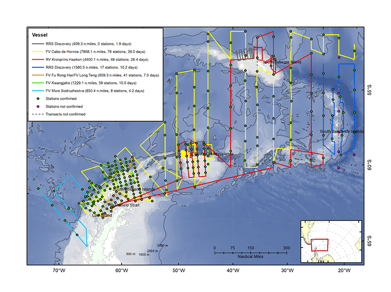
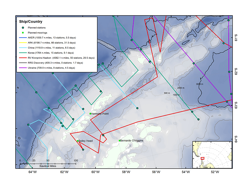
The CCAMLR-2000 Krill Synoptic Survey set out to estimate B0, in Subareas 48.1, 48.2, 48.3 and 48.4, and the associated estimate of error for the major area where commercial fishing takes place. The intention of the new Large-Scale synoptic survey was to repeat the 2000 survey by visiting the same areas using similar data collection methods (Hewitt et al. 2004; Watkins et al. 2004) for comparative analysis. The survey involved ships from Norway, ARK and Aker BioMarine AS, United Kingdom, Ukraine, Korea and China. A separate communication and planning e-group was established on CCAMLR website and CCAMLR WG ASAM and WG EMM meetings in 2018 have been arenas used for planning, coordination and standardization of methodology (Krafft et al. 2018 a,b, Knutsen et al. 2018, Macaulay et al. 2018).
Figure 1.1.Planned transect coverage to be surveyed by vessels taking part in the international krill synoptic survey in 2018/19.
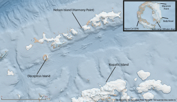
For the monitoring of land based krill predators, threeteams were deploy to three sites (2-3 people on each station) throughout Bransfield Strait (CCAMLR subarea 48.1); 1) Deception Island (Bailey Head) (62o 57' 52.90” S, 60o 29' 50.43”W), 2) Nelson Island (Harmony Point) (62o 17' 56.19” S, 59o 12' 56.76” W) and 3) Kopiatic Island off Bernardo O'Higgins (63o 18' 53.99”S, 57o 54' 39.44” W). These sites are key colonies for CCAMLR monitored krill predator species during their breeding season (Kokubun et al., n.d.; Naveen et al., 2012). Logistic support for the deployment of personnel was provided by the Norwegian cruise ship Hurtigruten (www.hurtigruten.no) for Deception and the Instituto Antártico Chileno (INACh) and the Chilean Navy for Nelson and Kopiatic Islands. The Chilean Navy and the Norwegian RV Kronprins Haakon provided the return of personnel from the field sites during late February 2019.
Figure 1.2. The location of the landbased predator field sites
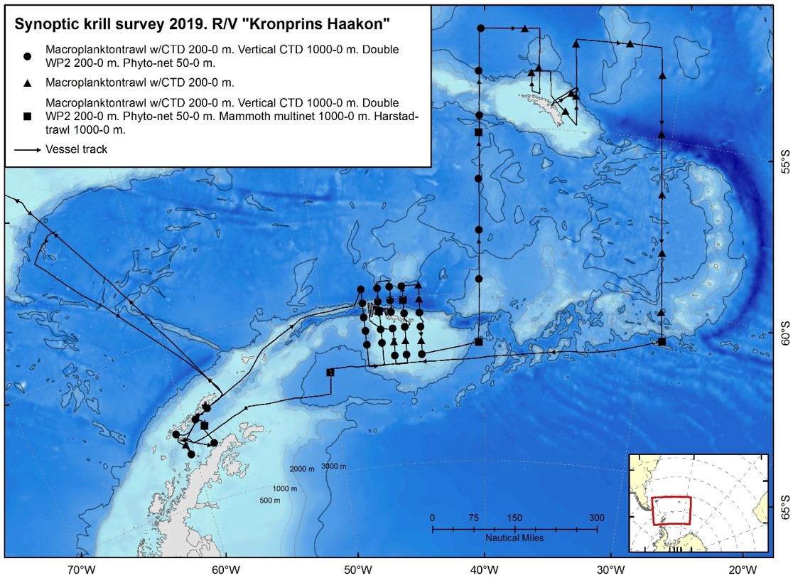
This report presents preliminary results from the survey performed with the Norwegian RV Kronprins Haakon between 08th January – 24th February 2019 (departure and return dates Punta Arenas, Chile) and the land-based predator research carried out between 21st November 2018 and 20th February 2019.
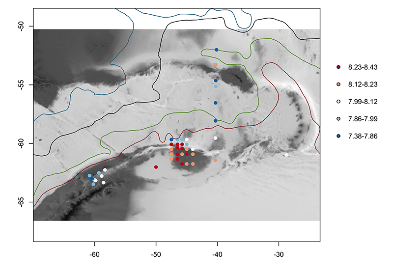
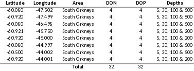
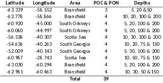
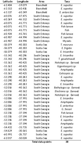
Figure 1.3. Summary of the 2019 krill monitoring survey performed with RV Kronprins Haakon.
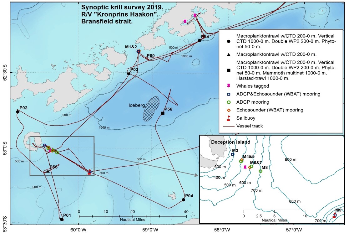
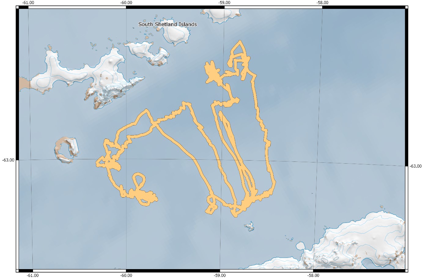
Figure 1.4. Summary of the activities in Bransfield Straight during the 2019 krill monitoring survey with RV Kronprins Haakon.
2 - Krill Acoustics
The synoptic krill acoustic survey was carried out as per the configurations, procedures, and plan in WG-EMM-18/12.
The drop-keel-mounted Simrad EK80’s onboard the vessel were used, operating at 18, 38, 70, 120, 200, and 333 kHz (Table 2.1) using version 1.12.2 of the EK80 software. These were calibrated on 16 January while anchored in Admiralty Bay, King George Island, as per normal procedures (Demer et al., 2015). The weather conditions were good, resulting in high quality calibration results on the main survey frequencies (RMS row, Table 2.1). The vessel’s ice-window protected Simrad EK80s were also calibrated on 16 January but were not used for survey operations.
To accommodate other acoustic instrumentation (ADCP, MS70 sonar), the pinging of the EK80 was controlled via the Simrad K-sync system. A nominal ping interval of 2 s was set with a 3-phase operation (ping EK80 and sonar, ping EK80 and sonar, ping ADCP, repeat). When the water depth was greater than about 1000 m, it was possible to ping the ADCP together with the EK80 and sonar without causing interference on the EK80, in which case all systems pung simultaneously at an interval of about 2 s.
The survey speed was nominally 10 knots, but in poor weather and shallow, poorly-charted areas, the vessel speed was reduced to as low as 5 knots.
The onboard quality control of the acoustic data were performed using the LSSS computer program (Korneliussen et al., 2006). Data were pre-processed using the KORONA program (Korneliussen et al., 2016) to detect and remove background noise as well as spike noise. However, the 38 kHz channel contained much spike noise that was not completely removed by KORONA and these were manually removed using the LSSS eraser tool along with any other extraneous noise or interference. The manual erasing was only done down to 300 m depth. The ship’s track that corresponded to formal survey transects was marked as so, but all acoustic data were scrutinized regardless of this. KORONA bottom picks were manually checked and adjusted as necessary. The bottom picks and integration regions were exported into Echoview format for subsequent krill detection and echo-integration as per CCAMLR procedures using Echoview.
For survey reporting purposes, the dB-difference method was used to select backscatter from krill. The dB-difference bounds were determined from the krill length frequency data obtained from trawls carried out during the survey. Distribution of krill NASC between a depth of 20 and 250 m was produced using the LSSS echo-integration exports on a nominal 514m horizontal and 5 m vertical grid from the 120 kHz channel.
Table 2.1. Survey configuration of the drop-keel-mounted EK80 echosounders.
Configuration/Channel
18 kHz
38 kHz
70 kHz
120 kHz
200 kHz
333 kHz
Transducer type
ES18
ES38B
ES70-7C
ES120-7C
ES200-7c
ES333-7C
Transmitted power (W)
2000
2000
750
250
150
50
Pulse duration (ms)
1.024
1.024
1.024
1.024
1.024
1.024
Absorption coefficient (dB km-1)
3.4
10.4
18.7
27.0
40.7
74.5
Sound speed (ms-1)
1456.0
1456.0
1456.0
1456.0
1456.0
1456.0
Sample distance (m)
0.041
0.058
0.070
0.058
0.047
0.035
Equivalent beam angle (dB)
-17.0
-20.70
-20.70
-20.70
-20.70
-20.70
Calibration gain (dB)
23.00
27.07
27.92
26.89
27.24
26.96
Beamwidths (alongship/athwartship)
10.1/10.5
7.0/7.3
6.6/6.7
6.7/6.5
6.5/6.2
5.7/5.7
Calibration RMS (dB)
0.14
0.24
0.08
0.09
0.20
0.81
Results
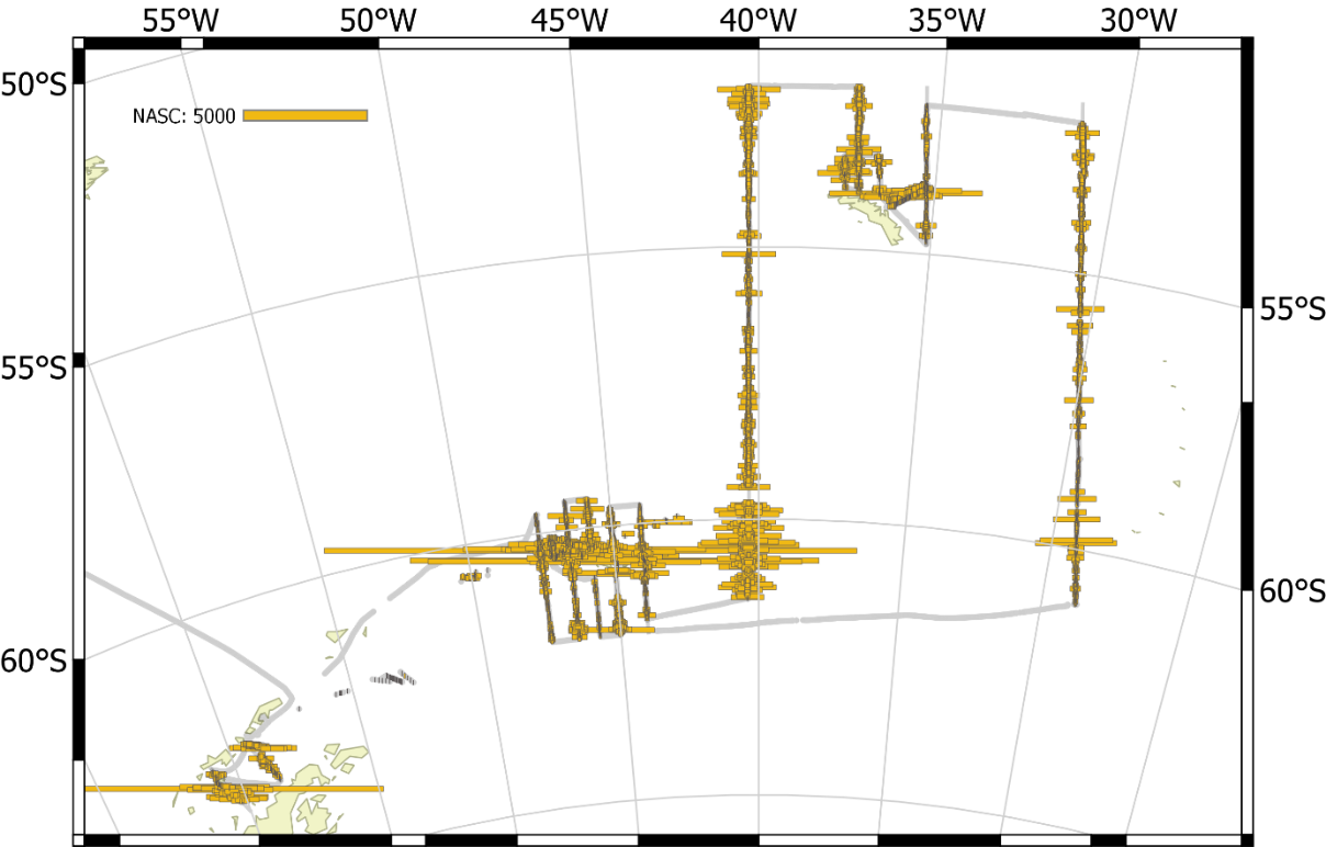
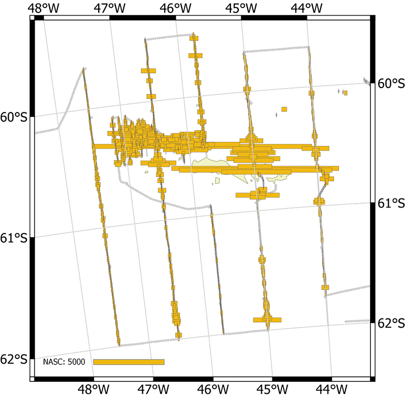
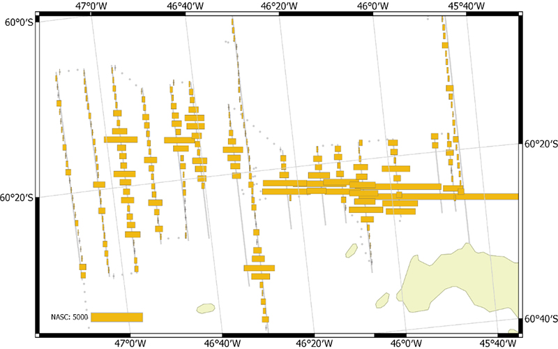
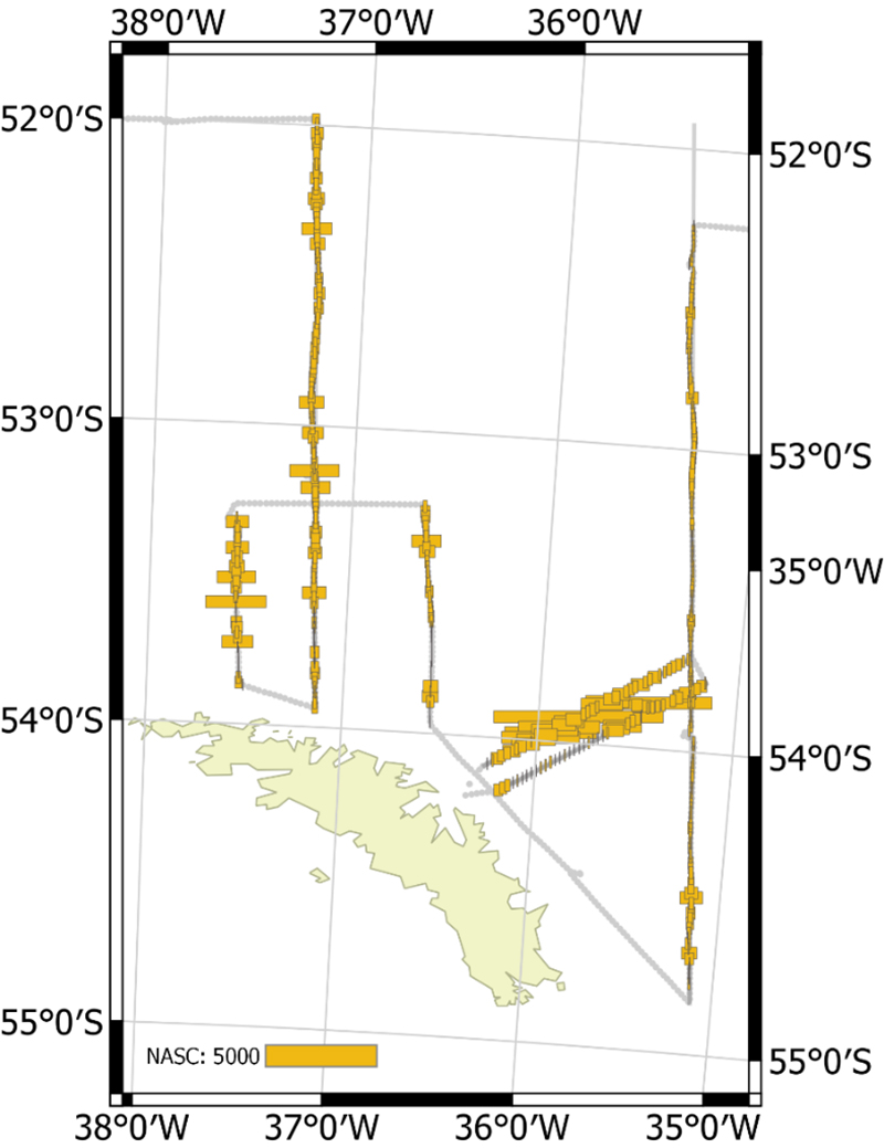
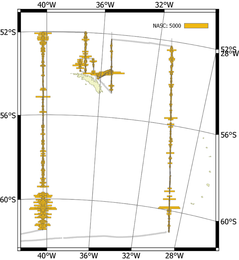
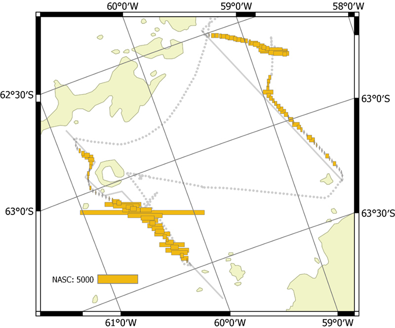
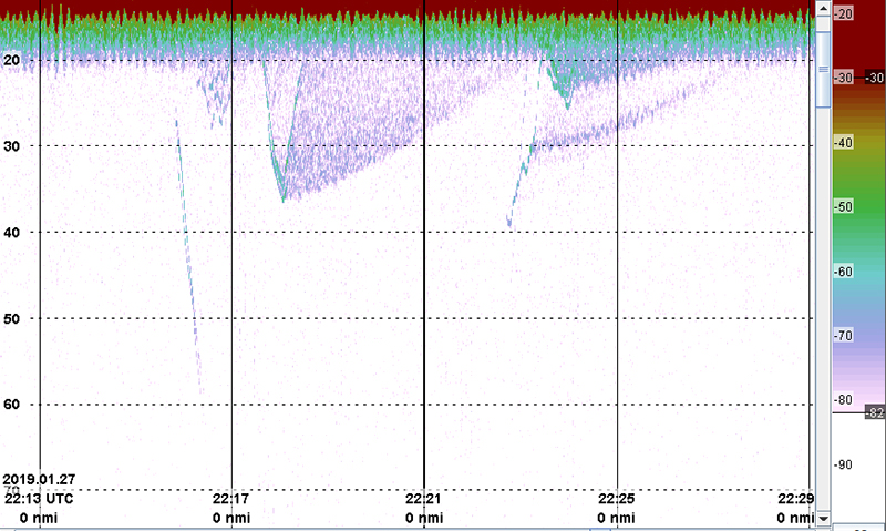
The vessel carried out all planned acoustic survey transects in the period of 18 January 2019 to 11 February 2019 (Table 2.2, Figure 2.1). The area of highest krill density was to the north and northwest of the South Orkney Islands (Figure 2.2, Figure 2.3). Most of the oceanic transects had few krill (Figure 2.2, Figure 2.4) except for the southern ends of the South Georgia transects (Figure 2.5). The Bransfield Strait saw moderate quantities of krill (Figure 2.6).
A large iceberg prevented full coverage of the most northerly transect in Bransfield Strait. The inshore end of some of the South Orkney Island transects were not covered due to uncertainties with bathymetry and small icebergs, as was the southern end of a Bransfield Strait transect. Ice did not significantly hinder any other parts of the planned transects.
No biomass estimate is presented here as this requires access to data from all the participating vessels, which will not occur until late May. The biomass results will be presented at the July 2019 CCAMLR SG-ASAM meeting.
Table 2.2. Start and stop times for the survey areas. The time periods include activities other than the acoustic surveying and hence do not reflect the actual surveying time.
Area
Start time (UTC)
End time (UTC)
Bransfield Strait
18/1/2019 10:30
20/1/2019 19:20
South Orkney Islands (wide area)
22/1/2019 20:10
31/1/2019 04:30
South Orkney Islands (high density)
26/1/2019 06:00
27/1/2019 12:10
South Georgia
1/2/2019 02:00
11/2/2019 19:50
Figure 2.1. NASC distribution from all transects carried out by Kronprins Haakon.
Figure 2.2. NASC distribution from the wide area transects around the South Orkney Islands.
Figure 2.3. NASC distribution from the high density transects to the Northwest of the South Orkney Islands.
Figure 2.4. NASC distribution from the transects to the North of South Georgia.
Figure 2.5. NASC distribution for the oceanic transect around South Georgia.
Figure 2.6. NASC distribution from the two transects in Bransfield Strait.
Additional acoustic measurements
The drop-keel-mounted EK80 echosounders were operated in broadband mode opportunistically during some of the CTD stations and in Admiralty Bay to collect target strength data from krill. These data have not been analysed.
The Simrad MS70 3D multibeam sonar was operated from 26 January until the end of surveying operations and was calibrated on 16 January. The MS70 was well-suited to detecting krill schools and could cover an entire krill school in one ping. At times, whales were also seen in the MS70 beam and hence has promise for observing the 3D motion of whales.
The Simrad ME70 multibeam sonar was operated at times in areas of high krill school densities, mainly for evaluation and testing purposes.
3 - Plankton, nutrients and environment
Along-track thermosalinograph data
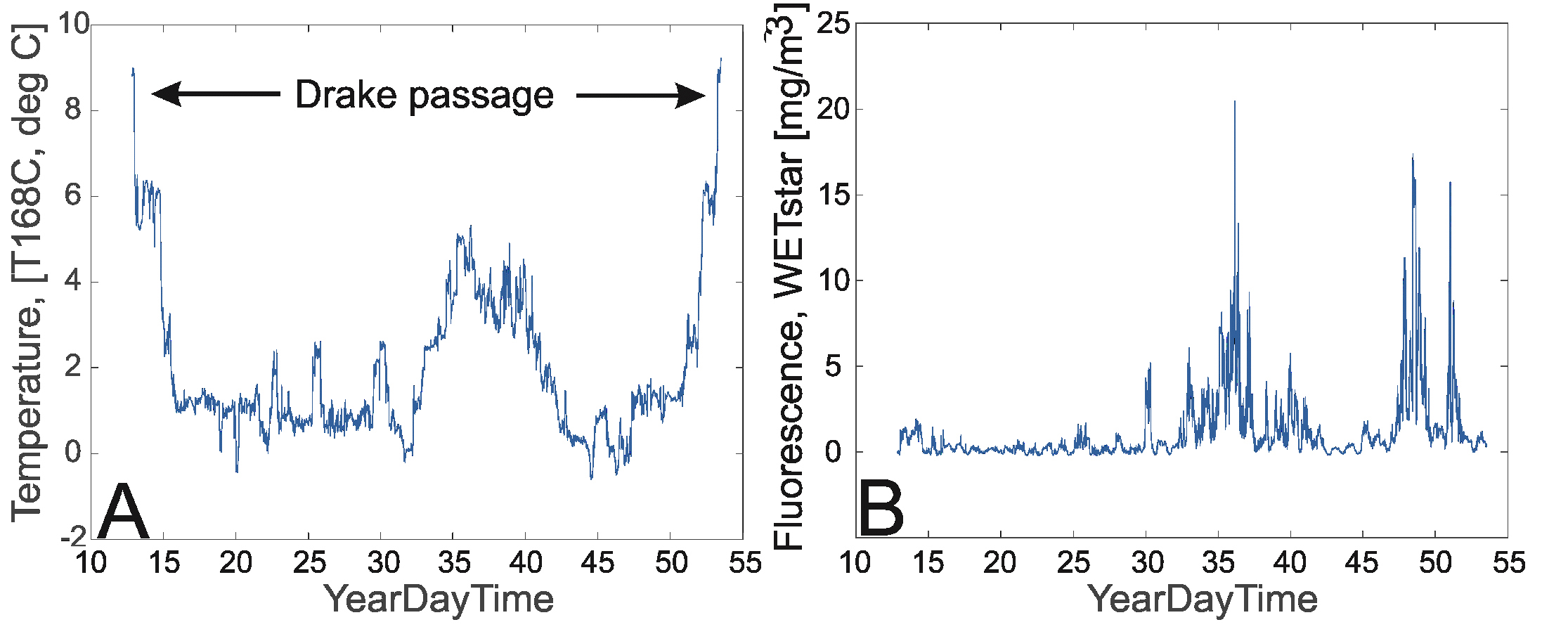
Temperature, salinity and fluorescence were recorded continuously along the complete track of the cruise using a ship-mounted thermosalinograph (SBE21). The real-time sample interval was 10 seconds. The water intake for the thermosalinograph is located about 4 m below the sea surface. The package holds two temperature sensors. The primary temperature sensor (sensorID =”55”) and the conductivity sensor (both with Serialnumber 3429) were calibrated 28 July 2017. A secondary temperature sensor is mounted close to the seawater intake. This sensor has a sensorID=”56”, but there is no information on calibration date in the cnv-files. There is a difference between the two temperature sensors, so that the primary sensor (sensorID=”55”) shows ~0.26-0.44°C higher values than the sensor close to the seawater intake. This seems to depend on the ambient temperature level. The data are noisy, and it should be investigated what caused this noise and how it can be best removed / filtered (see section on oceanography and thermosalinograph data).
A WET Labs WETstar fluorometer with factory calibration, calibration date of 20 June 2017 and a scale factor of 15.300 and blank output of 0.081 was used during the survey. Data output were in [mg Chl a/m3]. Since the factory calibration is more than 1 ½ year old, additional water samples for chl a and phaeophytin measurements were obtained from the same 4-m seawater intake as used by the thermosalinograph. This was done at irregular intervals in order to obtain a supporting set of chl a measurements that were used to make an in situ calibration of the WETstar fluorometer (cf. Table 3.1). The pigment concentrations (chl a and phaeopigments in µg L-1) were analyzed onboard the vessel (cf. Acknowledgements), using the fluorometric acidification method and a Turner Design AU10 fluorometer. Contrary to what is the procedure at IMR, the organic solvent was not acetone, but methanol, product #106009 from Merck, that is normally used by the Norwegian Polar Institute during joint the Nansen Legacy project, a protocol established for Arctic work.
Figure 3.1. A. Along-track temperature data, outer sensor (t168C) and B. Along-track fluorescence data for the period 12 January – 21 February 2019. From left to right, starting in Punta Arenas via the Drake passage to the Bransfield strait, South Orkneys, South Georgia and returning, again via the Drake Passage and back to Punta Arenas.
CTD on the pelagic trawls
A Seabird CTD, SBE37SM, was mounted on the headline of the pelagic trawls (Macroplankton and Harstad trawls) to obtain separate and additional data on the oceanography in the upper 200 m of the water column where the pelagic hauls were undertaken. These data are also used to visualize the trajectory of the trawl hauls and as support information when calculating volumes filtered during the Macroplankton trawl hauls. Both the temperature and conductivity sensors were calibrated on 20th of October 2018, while the pressure sensor was calibrated 23 October 2018.
Zooplankton sampling
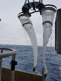
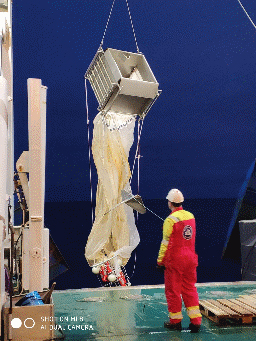
Sampling stations were performed along the survey lines every 12:00 and 24:00 hours (UTC). Mesozooplankton, macroplankton and micronekton were sampled with three different sampling systems: 1 - a double WP2 net (WP2DUO, Figure 3.2), 2 - a 1.0 m2 Multinet Mammoth system (HYDRO-BIOS Apparatebau GmbH -https://www.hydrobios.de/), and 3 - a Macroplankton trawl (Melle et al., 2006; Krafft et al., 2010; Heino et al., 2011), respectively.
1-The WP2DUO net pair was mounted on a single steel-frame with two rings holding the nets of 180µm mesh size. Zooplankton was sampled at most stations where the CTD-rosette collecting water samples for nutrients and chlorophyll was deployed (49 deployments – Table X1). The frame was attached to the end of the towing wire and the nets deployed vertically, usually to within 10 m of the seafloor if in shallow waters with bottom depths <200 m on the shelf and to 200 m depth on deeper stations. This corresponds to the maximum sampling depth when using the Macroplankton trawl (see below). The two samples were processed using standard IMR procedures. They were called WP2-A and WP2-B respectively, named after the marked A and B rings of the paired frame. The WP2-A sample was split in two and 50% was fixed in borax-buffered 4% formaldehyde for mesozooplankton identification and enumeration purposes. The other 50% was used for biomass estimation according to IMR standards (dryweight). This part was divided into 3 size fractions using sieves with mesh-sizes 2000, 1000 and 180 μm. The biomasses retained on the 1000 and 180 μm sieves were placed on separate pre-weighted aluminum dishes. The organisms retained on the 2000 μm sieve were sorted, counted and identified to different taxonomic groups; chaetognaths, amphipods, fish, krill, shrimps, the copepods Euchaeta sp., as well as a category called larger copepods (Copepoda) containing species such as Rhincalanus gigas, Calanoides acutus, Calanus propinquus. These groups were also put in separate pre-weighed aluminum dishes after lengths were measured of amphipods, krill, fish and shrimps. For the other categories number of organisms were counted. All the biological material from the size fractionation were also slightly rinsed in freshwater to remove excess salt prior to drying. Finally, the aluminum dishes were placed at 60°C degrees overnight, packed and stored in a freezer at -20°C degrees for later dryweight measurements onshore in the laboratory at IMR.
The other WP2 sample (WP2-B) was also split in two and 50% was preserved in 96% alcohol for later genetic analyses, while the second 50% subsample was fixed in borax-buffered 4% formaldehyde for identification and enumeration using FlowCAM. All these samples were imaged on board using two different FlowCAMs (see FlowCam analyses section). After imaging the samples were recovered and re-fixed in borax-buffered 4% formaldehyde. This was done in order to verify data obtained by the FlowCAM and to compare with traditional microscopy.
2 - The Multinet Mammoth system (Figure 3.3) with nine 180 μm meshed nets and sampling buckets, was used for stratified sampling to determine the depth distribution of mesozooplankton from 1000 – 0 m. Depth stratification was as follows, 1000-800m, 800-600m, 600-400m, 400-300m, 300-200m, 200-100m, 100-50m, 50-25m and 25-0m. The tows were oblique hauls and the ship speed was approximately 1.8-2.0 knots during the operation, while winch speed was 0.5 m/s during deployment and retrieval of the gear. The samples obtained using the Multinet were treated the same way as the WP2 samples (see above).
Figure 3.2. The WP2 DUO deployment from the CTD hangar of RV Kronprins Haakon 14 March 2019. Foto: Tone Falkenhaug, IMR.
Figure 3.3. Multinet Mammoth deployment from the stern of RV Kronprins Haakon 11 February 2019. Foto: Tor Knutsen, IMR.
The Macroplankton trawl (Melle et al., 2006; Wenneck et al., 2008; Krafft et al., 2010; Heino et al., 2011), was used to catch krill, mesopelagic fish and other macrozooplankton like salps, amphipods and cnidarians. This trawl has a ~36 m2 opening and a net with a mesh size of 3 mm (7 mm stretched), all the way from the trawl opening to the cod-end. The flow through the mouth opening of the trawl was measured acoustically with Scanmar sensors (TrawlSpeed / Symmetry) - sensors. In addition, Scanmar depth and door sensors were mounted to allow the full information on trawl depth, door spread, and geometry. The total catch was weighed, and the entire or subsamples of the catch (in cases of large biomasses) were sorted, weighed, and determined to the desired taxonomic resolution, usually to species level where possible. Some species/specimens were picked from the sample alive/freshly caught and preserved in 96% alcohol for genetic analyses. Other similar types of samples were fixed in 4% borax-buffered formalin.
If Euphausia superba were present in the trawl catch, the entire catch if small, or a subsample if large, was examined (up to ~200 individuals), and the body length of each individual krill was measured (± 1 mm) from the anterior margin of the eye to tip of telson excluding the setae, according to the “Discovery method” used in Marr (1962) and as also denoted AT (“anterior eye to tip of telson”, cf. Morris et al. 1988). Sex and maturity were determined for length-measured individuals using the classification methods outlined by Makarov and Denys (1981) based on external secondary sexual characters. Additional samples of E. superba were collected along the cruise track and were preserved on borax-buffered formalin (4%), or on 96% alcohol.
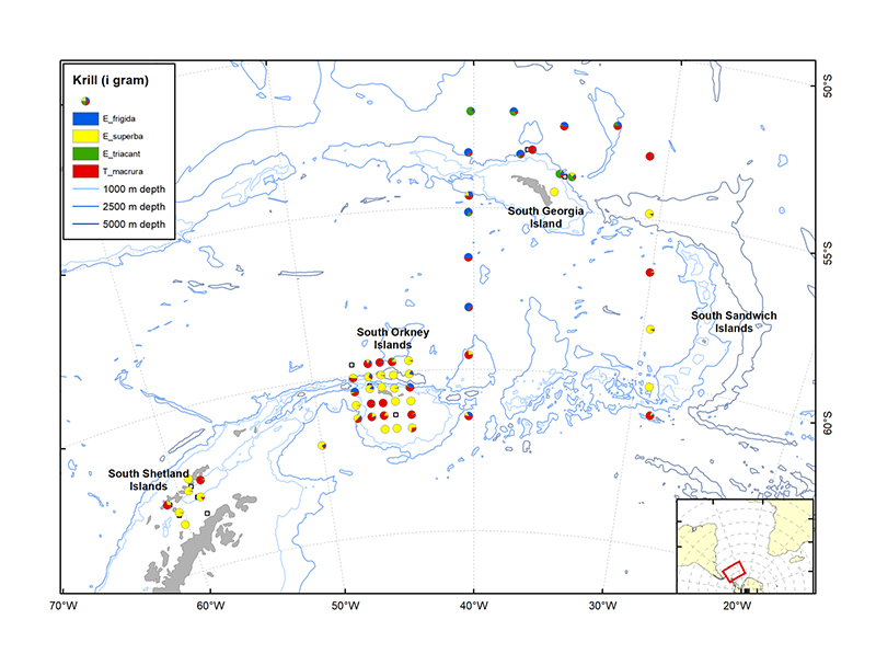
Figure 3.4. Distribution of the four krill species (Euphausia frigida, E. superba, E. triacantha and Thysanoessa macrura) sorted from trawl catches during the survey.
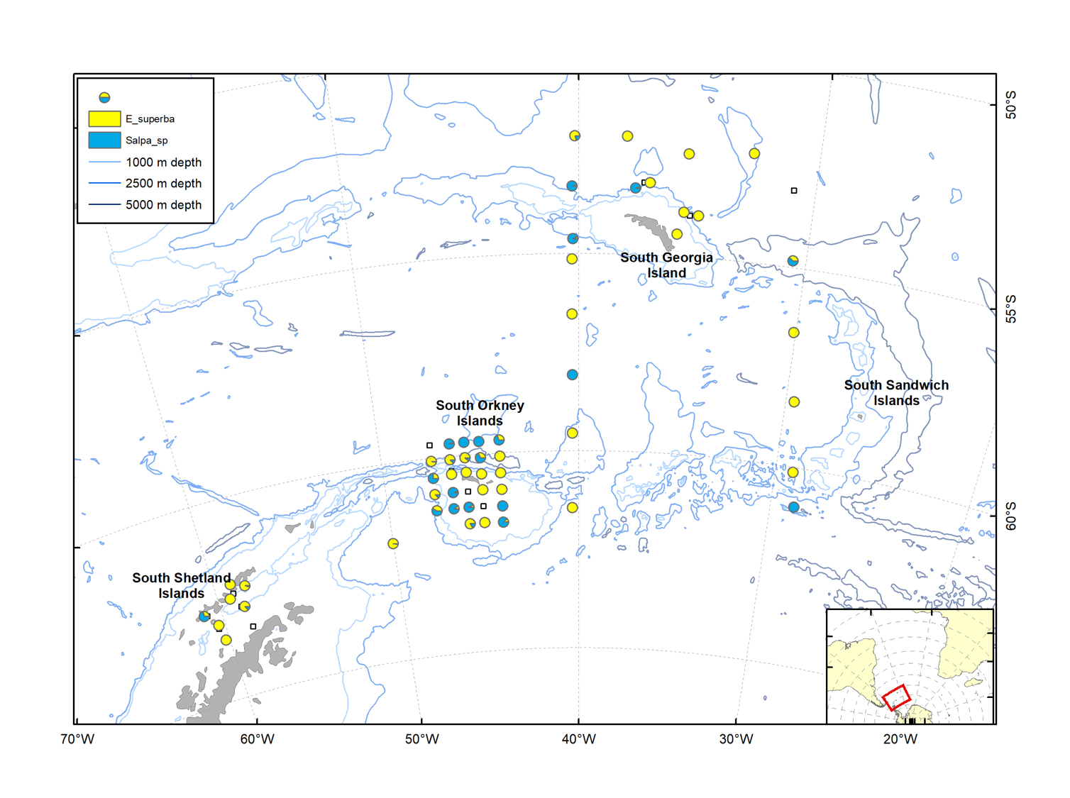
Figure 3.5. Proportional distribution of Euphausia superba (Antarctic krill) and Salpa thompsoni, sorted from trawls towed at predetermined stations.
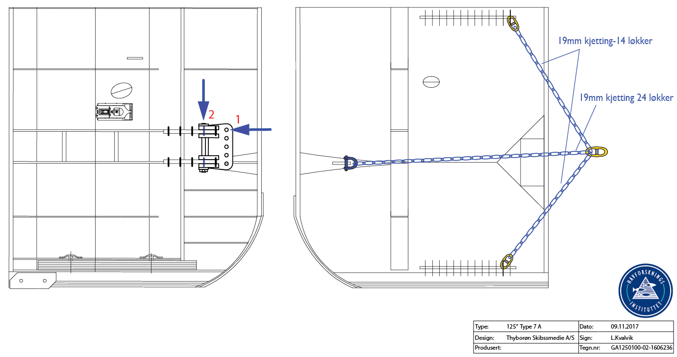
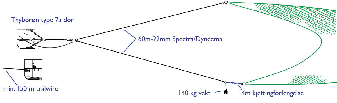
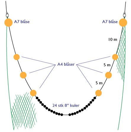
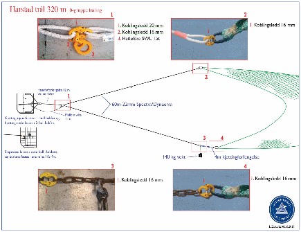
A standard pelagic Harstad trawl (Nedreås and Smestad, 1987; Godø et al., 1993; Dingsør, 2005) was operated regionally to approximately 1000 m depth in a V-haul allowing to obtain additional information on the taxonomic composition of the mesopelagic community, as well as fish larvae being associated with Euphausia superba over a somewhat extended depth range compared to the Macroplankton standard trawl hauls (200-0 m). Sex and maturity based on external secondary sexual characters as well as length measurements of Euphausia superba caught by the Harstad trawl was determined by the same methods as those used for the Euphausia superba Macroplankton trawl catches (see above). The Harstad trawl was equipped with an inner net of finer mesh. A description of the rigging and use of this Harstad trawl (in Norwegian) is given in Appendix 1.
Nutrients, phytoplankton and microzooplankton
Samples for nutrients (nitrogen, phosphate, and silicate) have been collected at 43 stations (CTD-stations), from the Bransfield Strait and the South Shetland islands in the south-west, to the South Orkneys and South Georgia islands in the north east. Samples (20 ml) were taken from Niskin bottles mounted on the CTD-rosette corresponding to standard depths from 1000 m to 5 meters, fixed using 0.2 ml of chloroform and stored at 4°C onboard the vessel. Nutrient analyses will be performed ashore at the after termination of the cruise using IMR standard analytical procedures.
Additionally, ca. 15-20 nutrient samples were taken from the water-intake associated with the thermosalinograph and FlowCam analyses of living phytoplankton and microzooplankton. Some of these nutrient samples were collected at short intervals when entering Whalers Bay at Deception Island (See FlowCam analyses section).
The concentration of chlorophyll a was used to estimate total phytoplankton biomass. 263 ml water samples were taken from Niskin bottles corresponding to 200, 150, 125, 100, 75, 50, 30, 20, 10, and 5-meter depth obtained by the CTD-rosette. A few stations had reduced sampling program due to weather, bottom depth or technical problems but chlorophyll samples were obtained from ca. 43 stations. The samples were filtered immediately after collection and the filters were stored frozen in the dark before analyses onboard the ship. Chlorophyll a and phaeopigments were analyzed fluorometrically using the acid addition technique (see above).
In addition, Fluorescence data were collected during each CTD cast (vertical distribution) using a WET Labs ECO-AFL/FL fluorometer attached to the CTD, but also continuously during the cruise via the thermosalinograph and the water intake at 4-m depth onboard the ship (horizontal distribution).
At each CTD station (43 stations) a quantitative combined phytoplankton and microzooplankton sample from 30 m depth was taken. Two brown 100 ml glass bottles were filled with seawater from the Niskin bottles corresponding to this depth and each was fixed with 2 ml lugol’s solution. Additionally, samples for qualitative phytoplankton and microzooplankton species analyses were obtained using a plankton-net (Algae-net) with mesh size of 10 µm hauled from 50-0 m depth at 0.1 m s-1 and fixed with 2ml 20% formaldehyde in a 100ml brown glass bottles.
The fixed quantitative and qualitative samples of phytoplankton and microzooplankton may be analyzed for species composition onshore according IMR standards using light microscopy at Flødevigen laboratory following the return of the ship to Norway. In addition, the fixed samples may be used to verify and implement the new FlowCAM technique. Effects of fixation (Lugols and formaldehyde) may be studied by comparing FlowCAM analyses of fixed material with analyses of live samples already imaged during the cruise (See FlowCAM section).
Table 3.1. The number of stations and samples collected are shown in the text table below.
Number of CTD stations
Nutrient samples[1000-5m]
Phytoplankton/ Microzooplankton samples from the thermosalinograph
Number of chlorophyl a samples from water bottles [200 - 0m]
Algae net hauls[0.1 m2, 10 µm]
Krill foraging experiments samples
[St3-51] 49
531
~40*
438
38
~20
Number of Multinet Mammoth hauls
Number of WP2DUO hauls[0.5 m2, 180 µm]
Phytoplankton/ Microzooplankton samples [30 m depth]
Number of chlorophyl a samples from the thermosalinograph
Harstad trawl [~1000-0m]
Macroplankton trawl [~200-0m]
6
39
~35**
28
8
59
*: Samples taken before the water intake-filter. More samples exist, but quality is uncertain.
**: On five CTD stations samples have been obtained from 3-4 additional depths.
Krill foraging experiments
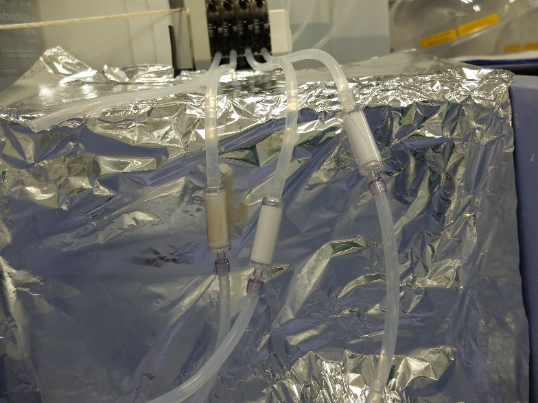
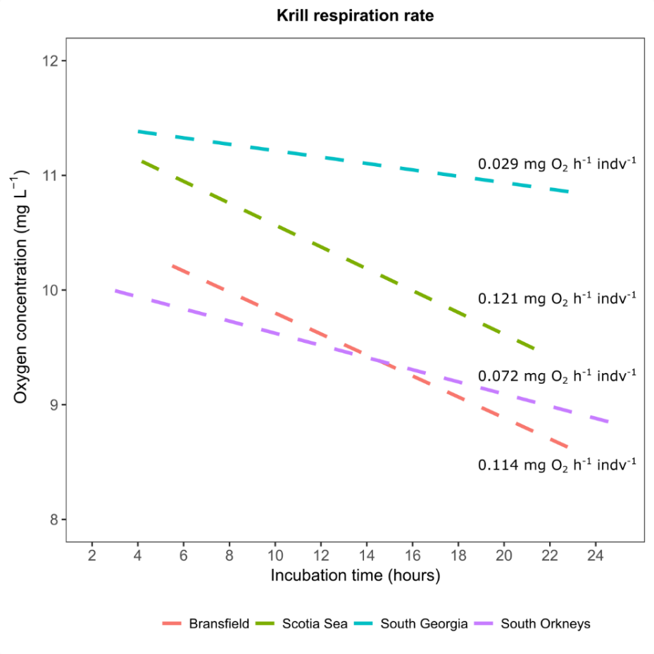
A few krill foraging experiments were conducted where individual krill were kept in 5-L glass bottles for 24-hours (see Juan Hofer). Before and after incubation the seawater was imaged using the FlowCAM macro. The analyses may be used to determine the effect of the presence of krill on the microplankton size-specter the > 50µm.
Fluorometer on the CTD
The fluorometer on the CTD is a FluoroWetlabECO_AFL_FL (Serial number : FLRTD-1547) with factory calibration date 1/4/2016.
4 - FlowCam studies
The FlowCam combines digital imaging and microscopy to analyze particles dispensed in fluids. Combined with automatic image recognition, the FlowCam have the potential to significantly effectuate data acquisition in routine monitoring programs. The instrument has been criticized for the small volumes of water it could analyze within a reasonable amount of time ((a few ml per hour)). However, the recently developed FlowCam Macro is designed to analyze much larger volumes at higher speeds than the original (several liters per hour). We brought both the original FlowCam Micro and the new FlowCam Macro to test the applicability of the instruments and to implement operation procedures for routine plankton monitoring cruises.
Aims and approaches
Microzooplankton/phytoplankton FlowCam procedure
The aim was to develop a FlowCam procedure to quantify and describe the microzooplankton and phytoplankton community in the photic zone.
Samples of seawater (3 liter) were taken at CTD stations from the 30-meter Niskin bottle and imaged using both FlowCam instruments. At selected stations samples from several depths including some in the euphotic zone were imaged. The samples were kept alive at 3.5 ᵒC in the dark and imaged within a few hours after collection.
All samples from 30 meter at the CTD stations were fixed in duplicate 100ml dark glass bottles using Lugol’s solution (2% final concentration) for later comparison of FlowCam and traditional light microscopy.
Several samples (72) were taken from the thermosalinograph (water inlet at 4 m depth) and imaged on both the FlowCam Macro and FlowCam Micro along the cruise line (info on samples can be obtained upon request). A selection of these samples were fixed in formaldehyde and lugol`s solution to verify size spectra, taxonomic classification and biomass estimations. To supplement FlowCam observations, animage library of observed species were made using an inverted microscope connected with camera (Figure 4.1).
Different combinations of flowcells (high precision glass cells for imaging) and objectives (2x, 4x and 10x) were tested on the FlowCam Micro while a 3x10mm flowcell and 0.5x objective was fitted to the FlowCam Macro (Table 4.1). Due to the low volumes imaged at high magnification (a few ml using the 4x and 10x objectives) with the FlowCam Micro, samples were concentrated by reverse filtration through a 20 µm mesh. Two to three liters of seawater was reduced to 50-150 ml concentrate and imaged for 10-60 minutes.
Mesozooplankton FlowCam procedure
The aim was to employ a FlowCam procedure to identify, quantify and describe the mesozooplankton community in the upper 200 meters at all CTD stations along the cruise lines and at selected depths at 6 different stations.
Samples obtained using a WP2-net and a Multinet Mammoth (sampling at nine different depths) equipped with 180µm mesh nets were fixed with borax-buffered formaldehyde (2% final concentration) and stored at 3.5 ᵒC before analyses. The fixed mesozooplankton samples were filtered through a 180µm mesh sieve to remove the formaldehyde and diluted in 2.5-3.0 L of freshwater for the FlowCam Macro analyses. Organisms were kept suspended in the sample container by gentle agitation and imaged at a flowrate of 200-375 ml min-1.
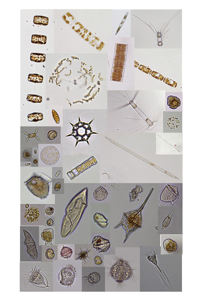
Figure 4.1. Phytoplankton and microzooplankton species observed during the cruise and imaged using an inverted microscope for verification of FlowCam images.
Higher magnification imaging was tested on mesozooplankton <1000µm by sieving away larger organisms through a 1000µm mesh sieve and using the FlowCam micro equipped with a 2x objective and 2x6mm flowcell. These samples were diluted with 600-1000ml of freshwater and kept suspended using a magnetic stirrer.
Preliminary results
Microzooplankton and phytoplankton
In general, there were low abundances and diversity in the phytoplankton and microzooplankton of Brandsfield Strait compared to the Scotia Sea and around the South Orkney Islands. In Brandsfield Strait the diatom Corethron penneatum and the dichtyophyte Dichyocha speculum dominated the phytoplankton while the tinntinid ciliate Epiplocylis sp. was the most common microzooplankton. The Scotia Sea and the waters around South Orkney Islands had high abundance and diversity of large diatoms. Rhizosolenia sp., Coscinodiscus sp. and chain forming species of Chaetoceros spp. were especially abundant (Table 4.1). As we passed through major hydrographic fronts, massive blooms of Rhizosolenia sp, Chaetoceos sp and Eucampia zodiacus were observed and studied using a combination of the thermosalinograph (measuring temperature, salinity and fluorescence) and FlowCam analyses.
Microzooplankton were only present in small amounts during the blooms of large diatoms. On the other hand, mesozooplankton were abundant and diverse. This indicates a short food chain from produces to larger consumers (mesozoo- and macroplankton). Thus, the Scotia Sea and the area around South Orkneys were associated with new production. Regenerated production dominated at the end of the cruise and in the Brandsfield Strait. Here, smaller phytoflagellates, oligotrich ciliates, heterotrophic and mixotrophic dinoflagellates were more abundant.
Figure 4.2. Snapshot of microplankton community in Whalers Bay, Deception Island imaged by FlowCam Micro. Large diatom chains and the colony forming Chaetoceros socialis were associated with large heterotrophic dinoflagellates and ciliates. Phaocystis antarctica was also present in this sheltered bay with high nutrient supply.
Surprisingly, the haptophyte Phaeocystis antarctica was only observed in a few stations. The Southern Ocean has previously been reported to alternate between two different states – one dominated by larger diatoms, the other dominated by Phaeocystis antarctica.
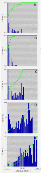
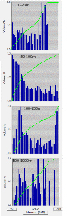
Figure 4.3. FlowCam size spectra of the microplankton community (10-200µm) as we approached and entered Whales Bay, Deception island. Samples were taken from the thermosaliograph at 4 meters depth. There was an abrupt change in the plankton community from outside (A,B), through the sound (C, D) to the interior the bay (E). Only 10 minutes of sailing between B and E.
The highest diversity and biomass of the microplankton community was observed within the sheltered Whalers Bay at Deception Island (Figure 4.2 and Figure 4.3). Here, large diatoms, Phaeocystis antarctica and several species of heterotrophic and mixotrophic dinoflagellates were observed. Whalers bay seems to be highly affected by a natural source of nutrient input of from the surrounding geology as a source for new production. Iron from the catchment area, underground geological activity and nutrients from the rich penguin and seal colonies may all be important factors in the fertilization of this sheltered bay. In contrast, the microplankton community in semi-sheltered bay at the neighboring King George Island was very low in abundance and dominated by small nanoflagellates and mixotrophic phytoflagellates. This bay is more affected by nutrient poor melting water of it`s large glaziers.
Table 4.1. Genera and species of microzooplankton and phytoplankton observed during the cruise, objective necessary for recognition using FlowCam images and their overall abundance
Group
Species
Recognizable with FlowCAM
Overall abundance (rank)
Microzooplankton
Tintinnid ciliates
Epipplocylis sp.
2x
4
Tinntinida indet.
2x
1
Oligotrich ciliates
Strombidium sp1.
2x
2
Strombidium sp2.
2x
2
Lohmaniella sp.
2x
2
Laboea sp.
2x
2
Heterotrophic dinoflagellates
Gyrodinium sp1.
2X
1
Nematodinium. Sp.
4x
1
Gymnodinium sp.
No
1
Peridinium steinii
10x
1
Protoperidinium sp.
10x
1
Mixotrophic dinoflagellates
Katodinium sp.
10x
2
Karlodinium sp.
10x
1
Dinophysis sp.
2x
1
Ceratium macroceros
0.5x
1
Ceratium sp.
0.5x
1
Mixotrophic cryptophytes
Teleaulax sp.
10x
1
Phytoplankton
Diatoms
Corethron sp.
0.5x
5
Rhizosolania spinifera
2x
3
Chaetoceros sp1.
2x
2
Chaetoceros sp2.
2x
5
Chaetoceros sosialis
0.5x
2
Melosira sp.
2x
2
Rhizosolaenia indica
0.5x
1
Eucampia zodiacus
0.5x
2
Rhizosolenia spinifera
0.5x
5
Chaetoceros curveticus
4x
2
Coscinodiscus sp.
0.5x
2
Nitcshia seriata
4x
5
Thallasiosira sp.
0.5x
2
Ceratulina sp.
2x
1
Dictyophytes
Dictyoca speculum
2X
3
Haptophytes
Phaeocystis antarctica
0.5x
1
Cooccolithophore indet.
no
1
Mesozooplankton
The mesozooplankton samples (WP2 and multinet) have been not been classified. A library of size-groups has is under construction and a taxonomy library for automatic classification will be created during the spring and summer.
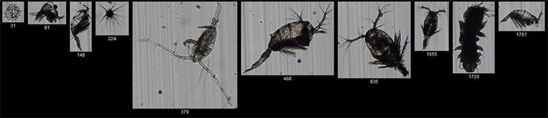
The FlowCam Macro produced high quality images for identification of genera and sometimes species of mesozooplankton of a size down to approximately 400µm (Figure 4.4). FlowCam Micro allowed identification of mesozooplankton from 100-1500µm to genera and sometimes species level. Mesozooplankton collected on a 2000µm mesh sieve should be analyzed using traditional microscopy, according to standard mesozooplankton procedure onboard during routine monitoring cruises at IMR.
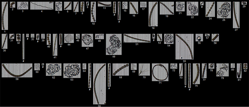
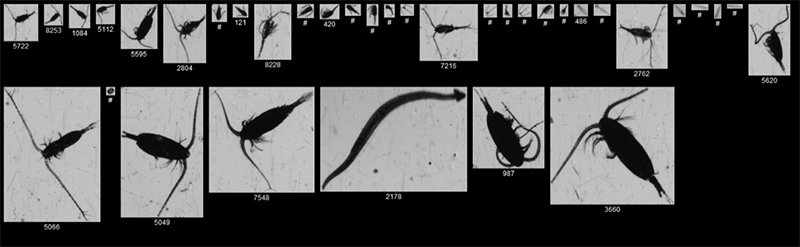
Figure 4.4. Examples of mesozooplankton images captured with the FlowCam Macro
Figure 4.5 Examples of mesozooplankton images captured with the FlowCam Micro
In addition to classifying and quantifying predefined groups, the FlowCam measures the size of hundred to thousand organisms. This allows the production of statistically strong size-spectra (Figure 4.3 and 4.6).
The samples obtained using the Multinet Mammoth were of poor quality. Several of the imaged individuals were not intact and the samples contained large amounts of animal debris. In contrast the individuals imaged from samples obtained using the WP2 net were of high quality with very little debris. We have suspected that the poor quality of Multinet samples were related to problems associated with flushing down the catch into the cups on deck. This results in different amounts of samples remaining in the nets that will be collected during the subsequent trawl. However, the poor quality of the sample was already observed in the first multinet trawl where unused nets were employed. An alternative explanation includes misplaced floats on the steel frame holding the cups of the multinet. These floats were mounted on top of the frame, and we do not know how it moves through the water. If the float brings the frame in a vertical orientation, the sample must pass through a constricted opening to reach the collecting cup. This issue needs to be addressed for the use of the Multinet Mammoth.
Figure 4.6. Example of size spectra of mesozooplankton from the multinet mammoth at station 45.
Regarding WP2-samples large amounts of diatoms created another problem for the analyses. A higher dark segmentation threshold for the camera capture (i.e.75) solved this problem. The small rest of diatoms images still captured will be filtered away using advanced filters in the software during post image processing.
Sample progression
All WP2 and multinet mammoth samples have been imaged using the FlowCam Macro (ca. 100 samples). The mesozooplankton size fraction from 180µm-1000µm has been imaged in about 30 samples using the FlowCam Micro at higher magnification (2x objective).
The samples of living microzooplankton, phytoplankton and mesozooplankton collected and imaged during the cruise must be processed by automatic classification software. This process will remove artifacts such as bubbles, debris and shadows. Thereafter, I will create a training set by manually assigning organisms into classification groups – taxa, organisms size and trophic role. This work has been initiated. I plan to use the most recent version of Zooimage, which is an R-package developed to classify digital images in general, and has been successfully employed to FlowCam, Video Plankton Recorder and Zooscan images (Alvares et al. 2012). In addition to classifying and quantifying organisms into predefined taxonomically, functional or size-groups, plankton size spectra will be created. These will be based on hundreds-thousands of individuals, a process that is impossible using traditional microscopy.
An overview of imaged samples may be provided upon request.
Conclusion
The FlowCams operationality at sea was much higher than expected. There were no problems with ship-movement and vibrations and analyses could be run in bad weather (strong gale). This may be because RV Kronprins Haakon is a large and heavy ship little affected by waves. The FlowCam Macro procedure developed during this cruise for identification and quantification of mesozooplankton may stand alone, while combining the FlowCam Micro with observations using an inverted microscope significantly increase the taxonomic resolution for phytoplankton and microzooplankton.
5 - Fish and Cephalopods
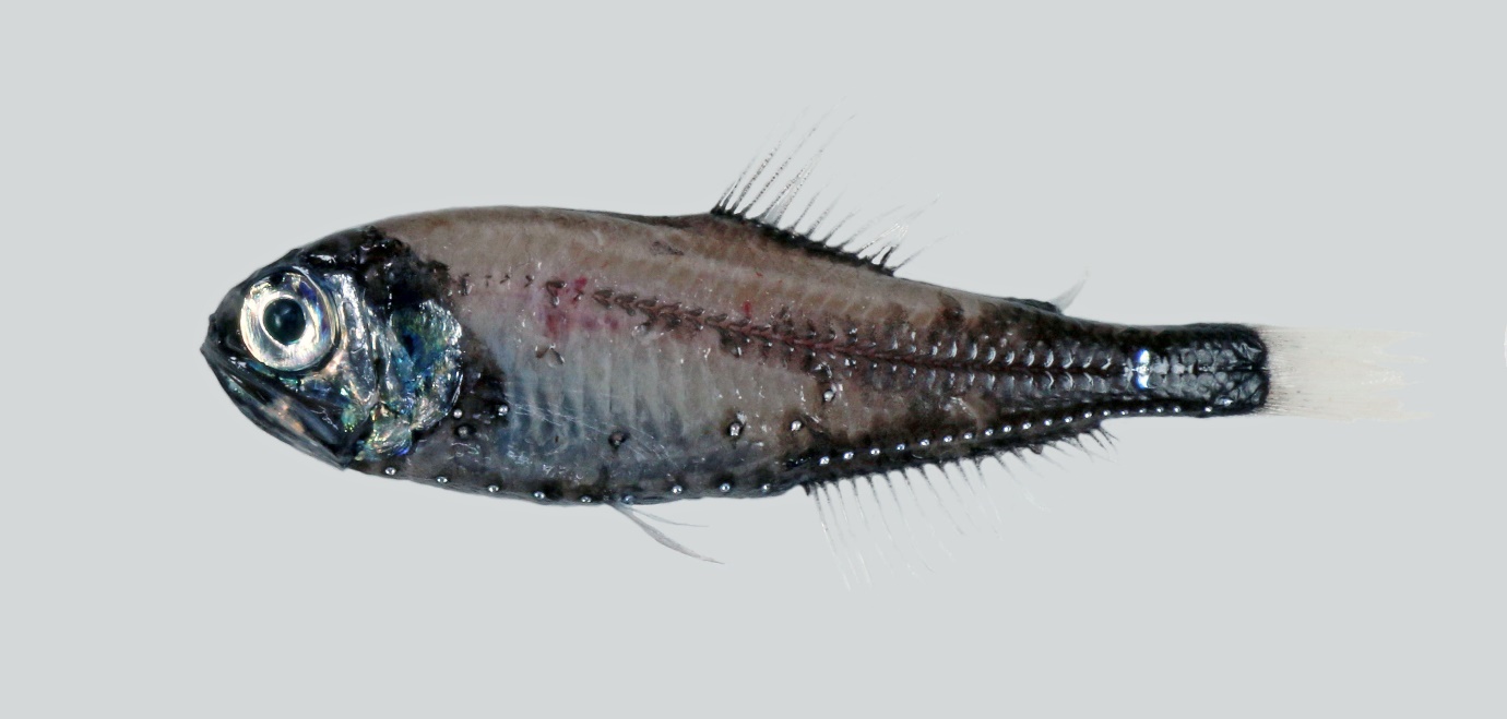
Two different trawls were used, the microzooplankton trawl towed from 200 m depth to the surface and the Harstadtrawl towed from 1000 m depth to the surface. All fishes and cephalopods were sorted from the catch, identified to highest taxonomic level possible, and length measured. Standard lengths were taken of all argentini-, stomii-, aulopi-, and myctophiform fishes, total lengths of the remaining orders of fishes, mantle length of cephalopods. Lengths were measured to the mm below (larvae/juveniles and standard lengths), or to the 0.5 cm below (total and mantle lengths). Total weight was taken per taxon and station. Genetic samples for selected taxa were preserved in ethanol and voucher specimens frozen. Four species of myctophids (Electrona antarctica, Gymnoscopelus fraseri, Krefftichthys anderssoni, and Protomyctophumbolini) were sexed based on external characters (presence of supra- and infracaudal luminous glands, or shape of the antorbital luminous organ). Species identification was primarily based on Gon & Heemstra (1990) (adult fish), Kellermann (1990) (fish larvae), and Jereb & Roper (2010) (cephalopods). In addition, various other taxonomic literature and webpages were used to secure correct identification.
Results
Fish
A total of 4,941 specimens (7.5 % larvae) were caught in 47 macroplankton- and eight Harstadtrawl hauls. These belonged to 9 orders, 17 families, and 53 taxa on species or genus level (Table 5.1). The dominating taxa, both in number of specimens and biomass, were the two lanternfishes Electrona antarctica (Figs. 1 and 2) and Gymnoscopelus braueri, and the deepsea smelt genus Bathylagus. As expected, diversity was highest in the deep hauls conducted with the Harstadtrawl. In the macroplankton hauls however, fish diversity and biomass were higher during night than during day, evidencing the diel vertical migration of the mesopelagic species. Daytime hauls with the macroplankton trawl resulted almost exclusively in only fish larvae or no fish catch, although invertebrates were always present.
Some specimens could not be identified to species level for the time being. This was due to insufficient identification keys, especially since not all larval stages are described for all species yet (Kellermann 1990). This applies especially to perciform larvae. However, it seems very likely that larvae of Electrona sp. and Notolepis sp. are offspring of the dominant and widespread E. antarctica and the only barracudina-species registered, N. coatsi, respectively. The leptocephali larvae of the order Anguilliformes belong, based on number of myomeres, probably to the snipe eel family Nemichthyidae, possibly Labichthys sp. The genus Bathylagus poses some taxonomic challenges with partly contradicting identification keys. Most of these specimens were frozen for closer examination in the lab on land. Genetic samples of all taxa not identified to species level were taken.
Table 5.1. List of fish taxa caught during the survey, divided into adults and larvae/juveniles; total number of trawl stations with taxon present (N1) and of specimens registered (N2), biomass (total weight) in kg (BM), presence in macroplankton- (M) and Harstadtrawl (H). Data are not corrected for water volume filtered.
adults
larvae/juveniles
Order
Family
Species
N1
N2
BM
M
H
N1
N2
BM
M
H
Anguilliformes
indet.
2
2
0.010
x
Argentiniformes
Microstomatidae
Nansenia sp.
1
2
0.072
x
Bathylagidae
Bathylagus sp.
13
737
11.162
x
x
3
4
0.000
x
Stomiiformes
Gonostomatidae
Cyclothone microdon
4
20
0.021
x
Stomiidae
Borostomias antarcticus
2
9
0.328
x
Aulopiformes
Scopelarchidae
Benthalbella elongata
1
3
0.128
x
Paralepididae
Notolepis coatsi
9
124
3.619
x
x
Notolepis sp.
25
128
0.022
x
x
Myctophiformes
Myctophidae
Electrona antarctica
27
2035
14.476
x
x
Electrona carlsbergi
4
122
0.919
x
Electrona sp.
9
38
0.003
x
Gymnoscopelus bolini
4
6
0.502
x
Gymnoscopelus braueri
23
866
7.245
x
x
Gymnoscopelus fraseri
8
75
0.267
x
Gymnoscopelus microlampas
3
3
0.065
x
x
Gymnoscopelus nicholsi
24
133
2.929
x
x
Gymnoscopelus opisthopterus
5
133
3.276
x
Gymnoscopelus piabilis
2
15
0.287
x
Krefftichthys anderssoni
11
128
0.353
x
x
Lampanyctus achirus
3
5
0.103
x
Protomyctophum andriashevi
2
3
0.005
x
Protomyctophum bolini
14
59
0.098
x
x
Protomyctophum choriodon
1
1
0.003
x
Protomyctophum tenisoni
1
4
0.002
x
Gadiformes
Muraenolepididae
Muraenolepis sp.
8
40
0.008
x
Macrouridae
Cynomacrurus piriei
2
2
0.099
x
2
2
0.001
x
adults
larvae/juveniles
Order
Family
Species
N1
N2
BM
M
H
N1
N2
BM
M
H
Scombriformes
Gempylidae
Paradiplospinus antarcticus
6
17
1.025
x
x
Centrolophidae
Pseudoicichthys australis
1
1
0.708
x
Pleuronectiformes
Achiropsettidae
Mancopsetta maculata
1
1
0.026
x
Perciformes
Nototheniidae
Aethotaxis mitopteryx
1
3
0.267
x
Lepidonotothen kempi
4
5
0.007
x
x
Lepidonotothen larseni
2
4
0.139
x
3
28
0.048
x
Lepidonotothen sp.
2
4
0.004
x
Notothenia coriiceps
5
8
0.001
x
Notothenia neglecta
1
1
0.000
x
Notothenia rossii
4
9
0.013
x
Pleuragramma antarctica
4
17
1.043
x
Pseudotrematomus loennbergii
3
3
0.001
x
Trematomus sp.
1
2
0.017
x
indet.
3
3
0.002
x
Artedidraconidae
Artedidraco skottsbergi
1
1
0.000
x
Artedidraco sp.
2
13
0.005
x
Pogonophryne sp.
1
1
0.000
x
Bathydraconidae
Gymnodraco acuticeps
1
1
0.061
x
Prionodraco evansii
4
7
0.002
x
Channichthyidae
Chaenocephalus aceratus
1
1
0.040
x
8
23
0.046
x
Chaenodraco wilsoni
4
7
0.008
x
x
Chionodraco rastrospinosus
3
24
0.379
x
12
29
0.015
x
x
Cryodraco antarcticus
1
1
0.008
x
4
12
0.008
x
x
Dacodraco hunteri
1
1
0.011
x
Neopagetopsis ionah
5
13
2.558
x
x
Pagetopsis sp.
2
2
0.001
x
Pseudochaenichthys georgianus
2
2
0.000
x
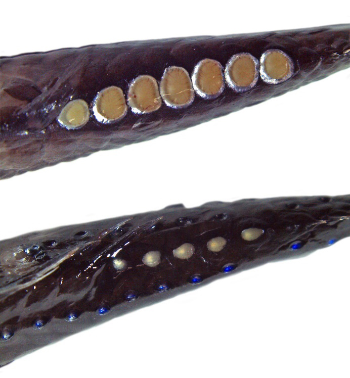
Figure 5.1. Electrona antarctica, female, caught on 22 January at 60°04.55’S 47°28.14’W in 29-202 m depth, 95 mm standard length. Photo: Merete KvalsundFigure 5.2. Sexdimorphism in Electrona antarctica: supracaudal (SUGL) and infracaudal (INGL) luminous glands; (top image) SUGL (consisting of 7 separate glands) on the dorsal side of the caudal peduncle of a 86 mm male, dorsal adipose fin showing in front of gland; (lower image) INGL (consisting of five separate glands) on the ventral side of the caudal peduncle of a 91 mm female, posterior anal fin rays showing in front of gland, also showing the posterior anal and precaudal photophores, those on the right side of the body with blue glimmer. Photos: Merete Kvalsund
Cephalopods
Table 5.2 lists data on cephalopods caught in 18 macroplankton and five Harstadtrawl hauls. All belonged to the order Oegopsida, except B. abyssicola which is not assigned to any order. Due to its small size (8 mm) one specimen could not be identified for the time being. Lengths varied within species, with a tendency of larger specimens taken in deeper hauls or during night. All specimens were kept frozen.
Table 5.2. List of cephalopods caught during the survey; total number of trawl stations with species present (N1) and of specimens registered (N2), biomass (total weight) in kg (BM), presence in macroplankton- (M) and Harstadtrawl (H). Data are not corrected for water volume filtered.
Family
Species
N1
N2
BM
M
H
Brachioteuthidae
Slosarczykovia circumantarctica
15
44
0.249
x
x
Chiroteuthidae
Chiroteuthis sp.
1
1
0.050
x
Cranchiidae
Galiteuthis glacialis
11
22
0.853
x
x
Psychroteuthidae
Psychroteuthis glacialis
3
4
0.094
x
indet.
1
1
0.000
x
Bathyteuthidae
Bathyteuthis abyssicola
2
3
0.043
x
6 - Marine mammals and birds
Marine mammal and bird (penguin) sightings were carried out by two dedicated observers during daylight (0600–2000 local time) along all survey transects, including during trawling. Periods on effort during transects and trawling were given different effort categories, so that they could later be treated differently. Periods on transects and during trawling (at very low speed) were analyzed using point and line transect approaches respectively. The observation platform was ca. 25 m above sea level (9th deck on KPH), and due to obstructed view to Starboard (due to various navigational installations), dedicated observations were usually made within the Forward Port Quarter (270-360 degree), covering targets out towards the horizon. However, dedicated observers also scanned outside of this sector, and occasionally recorded dedicated observations also within the part of the Forward Starboard Quarter that was not obstructed. Because the observation platform was located 50 m from the bow and 10 m from Port side, the blind-zone towards the bow and Port side were ca. 70 and 30 m, respectively. Incidental sightings, from other people on the observation deck or from dedicated observers while off effort, were also recorded. Each recorded observation included the following parameters:
Species
Group size
Distance to target at first sighting
Bearing relative to the bow of the vessel
Time (UTC)
Vessel’s position (automatically via GPS interface)
Weather and sea conditions were continuously monitored every 15 minutes, or when conditions changed dramatically. In addition, data were extracted from the ship’s weather and cruise log, to validate the observations recorded by the observers and to provide more continuous information every minute. Records were made using an in-house voice recording system which contains a microphone and a GPS connected to a laptop. The system records vessel position and time every 5 minutes, and a .wav sound-file is generated each time a sighting is read into an activated microphone. Observations were carried out using the naked eye for spotting and through binoculars for identification. In the case of species uncertainties, a rage of categories were used, such as: ‘large cetacean’, ‘large baleen whale’, ‘like fin whale’, ‘like humpback whale’. In cases where subsequent re-sightings lead to a definite species identification, these re-sights were matched to the original sighting, providing information about the distance at which positive identification could be carried out, relative to the distance of the original sighting.
Satellite tagging & biopsy sampling
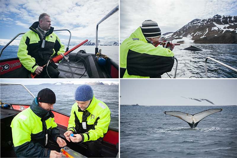
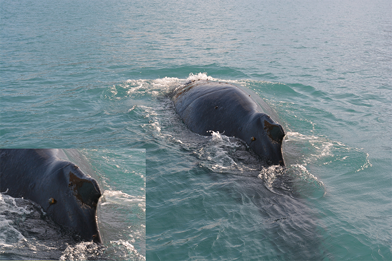
Three whales were equipped with Wildlife Computers location-only satellite transmitters (Limpet, SPOT-240-C). The transmitters were attached with two six-petal titanium dart anchors (68mm L x 24mm W x 6g), which were disinfected prior to deployment using Chlorhexidine. The Limpet tags were deployed using carrier dart which was fired from a pneumatic rifle (ARTS, Restech A/S, Figure 6.1). The carrier bounced back upon impact and could subsequently be retrieved from the water to for re-use. All tagging work was done from a Polarsirkel 23 ft work boat from the R/V ‘Kronprins Haakon’. The first Limpet tag was deployed on a fin whale in Admiralty Bay, King George Island, on Jan 16, 2019, while the second tag was deployed on a humpback whale just SE of Deception Island on Jan 19th (Figure 6.2). The third tag was deployed in Admiralty Bay on Feb 18th, but upon writing this report no uplinks had yet been received. One likely reason for this is that electrical tape (which was used to hold the tag in place on the carrier) remained in place on the tag, trapping saltwater between the saltwater switch electrodes and thereby disabling transmissions.
Biopsies of skin (and some blubber) were obtained from 10 humpback whales, using hollow biopsy tips (40mm L x 6mm D) held by biopsy darts fired from the same rifle that was used for satellite tagging (Figure 6.1). Samples will be used for DNA analyses and will also be tested for the presence of bacterial material.
In addition to tagging and collecting biopsies, photo-ID images were also collected, both during tagging/biopsy operations onboard the work boat, or by dedicated observers, other researchers and crew from onboard the “Kronprins Haakon” (Figure 6.1). Images will be used in conjunction with DNA analyses, and will also be submitted to the ‘Happy Whale’ online photo ID portal [https://happywhale.com/].
Figure 6.1. Top left: Cruise leader and the ARTS tagging and biopsy rifle; Top right: Dart being fired towards a humpback whale (note the orange dart visible just behind the dorsal fin); Bottom left: Preparing a collected biopsy for storage; Bottom right: Photo-ID image of one of the biopsied humpback whales. (All photos: Oda Linnea Brekke Iden)
Figure 6.2. Wildlife Computers Limpet satellite tag deployed just below the dorsal fin on a humpback whale. (Photo: Bjørn Krafft)
Results
Visual observations
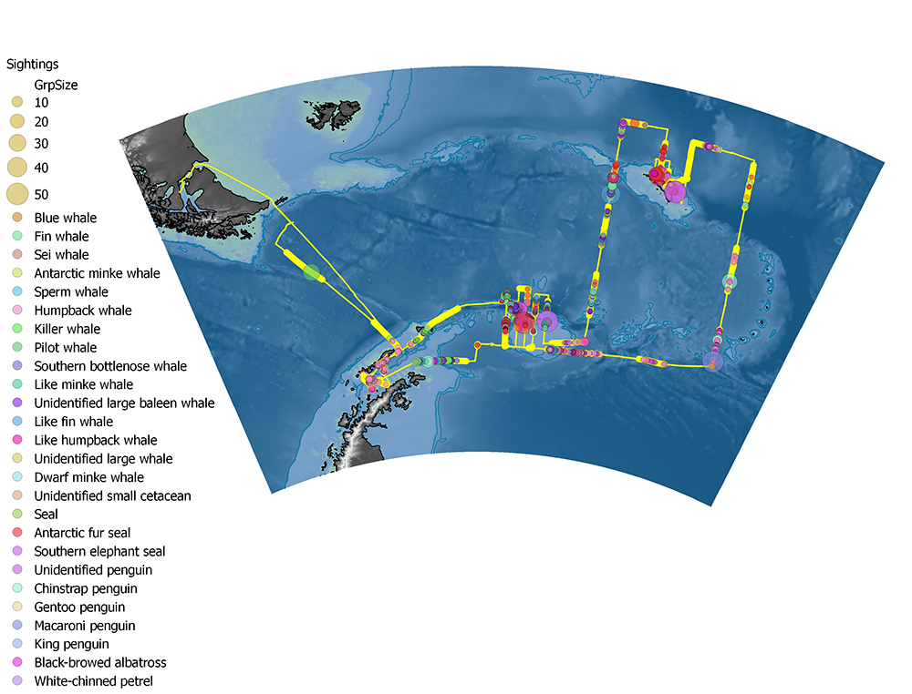
The sighting conditions (weather, visibility and sea state) were highly variable throughout the cruise; sea state varied between Beaufort 0 and 7, and fog or snow patches often limited the visual range. Dedicated observations were carried out for a total of 294 hours out of a total cruise duration of 1031 hours. We made a total of 927 primary sightings of 2504 individuals, covering 24 marine mammal and penguin species. A total of 1241 whales, 670 seals and 492 penguins were recorded (Table 6.1). Humpback and fin whales were by far the most dominant species; humpback whales dominated in Bransfield strait, and along the north coast of South Georgia, while fin whales dominated around the South Orkneys (Figure 6.3). Large mixed groups of fin and humpback whales were recorded in a region southwest of South Georgia, in a distinct patch to the NE of South Georgia, and along the southern flank of the shelf break south of the South Orkneys.
Table 6.1. Number of individual animals observed by species
Species
N
Antarctic blue whale
9
Fin whale
359
Sei whale
10
Antarctic minke whale
9
Sperm whale
1
Humpback whale
296
Killer whale
7
Pilot whale
30
Southern bottlenose whale
5
Like minke
1
Unidentified large baleen whale
219
Like fin whale
235
Like humpback whale
52
Unidentified large whale
7
Dwarf minke whale
1
Unidentified small cetacean
1
Antarctic fur seal
669
Southern elephant seal
1
Unidentified penguin
257
Chinstrap penguin
114
Gentoo penguin
13
Macaroni penguin
105
King penguin
3
Figure 6.3. Distribution of sightings along cruise track. Fat yellow line represents periods when observers were on effort.
Satellite tagging & biopsy sampling
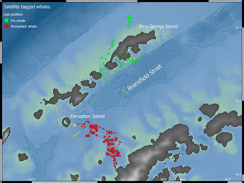
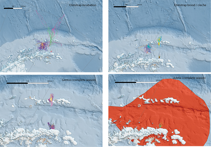
Figure 6.4 shows the tracks of the two satellite tracked whales within the Bransfield Strait area. The fin whale tag reported positions for a period of 12 days, from initial tag deployment in Admiralty Bay on Jan 16th until the last position was received from the shelf to the north of King George Island on Jan 28th. During this period, the whale initially travelled into Maxwell Bay, where it remained for 2 days. The whale then travelled to a shallow water spot outside a glacier face along the coast between Admiralty and Maxwell Bay. It appeared to alternate between periods within this shallow water region and a second region in deeper waters slightly offshore, until it travelled back and forth twice through the sound between King George and Nelson Islands, before finally seemingly heading north towards the shelf break. Unfortunately, we lost contact with the tag shortly thereafter.
The humpback whale that was tagged on Jan 19th just SE of Deception Island travelled in a generally southward direction (Figure 6.4). It initially followed relatively closely the transect taken by “Kronprins Haakon” towards the SE, before the whale ventured farther west and south towards the Trinity Peninsula on mainland Antarctica. The whale appeared to alternate between focusing in several distinct regions and transiting between these regions. The whale then travelled back towards the north, where the signals were lost on Jan 29th, very close to the original tagging position.
Figure 6.4. Tracks from the two satellite tagged whales, showing their movements within the Bransfield Strait region over a period of 12 and 11 days for the fin and humpback whale respectively. Note the overlap in movements by the humpback with the sampling transect line (yellow) followed by “Kronprins Haakon” during the days immediately after tag deployment
Biopsies were collected from 10 humpback whales. Five of these were collected in Admiralty Bay on King George Island while the other five were collected SE of Deception Island, in both cases in connection with satellite tagging operations. Except for one short excursion to the SW of the South Orkneys, we were unable to conduct tagging and biopsy operations outside of Bransfield Strait. This was due to the crew being short-staffed for operations while on station, meaning that crew were unavailable as boat drivers.
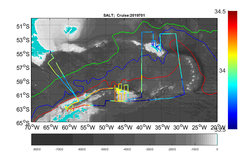
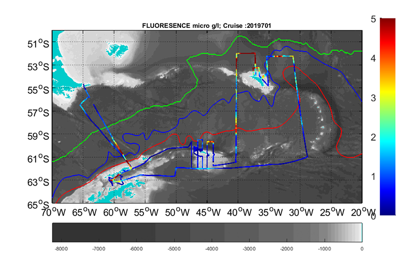
7 - Thermosalinograph and ADCP data
On a dedicated water intake a SBE 21 SeaCAT thermosalinograph was monitoring the temperature, salinity and fluorescence. The intake was at 4m depth. Close to the intake a SBE38 temperature sensor was mounted and measured the temperature unaffected by heating by the flow of water inside the ship. The fluorescence was measured by a WET Labs WET star fluorometer. The SeaCAT ran continuously during the survey obtaining samples every 10 seconds. A filter at the intake prevented biological material to enter the SBE 21 SeaCAT, but high concentrations of krill and other planktonic material caused a reduced flow at times. This caused increased short term variability in the salinity measurements. It is unknown if it caused biases in the measured salinity, but we will look further into it, by calibrating against drawn water samples from the pumped system and regular CTD station.
Spikes were removed by filtering with an hour long running mean filter and removing points with large deviations from this value. After the outliers were removed the original series were filtered with the same one hour running mean filter and subsampled at one minute resolution.
Along track values of temperature (intake), salinity and fluorescence are presented in figure 7.1.a, b and c.
Figure 7.1 a) Along track temperature at 4 m depth.Figure 7.1 b) Along track salinity at 4 m depth.Figure 7.1 c) Along track fluorescence at 4 m depth.
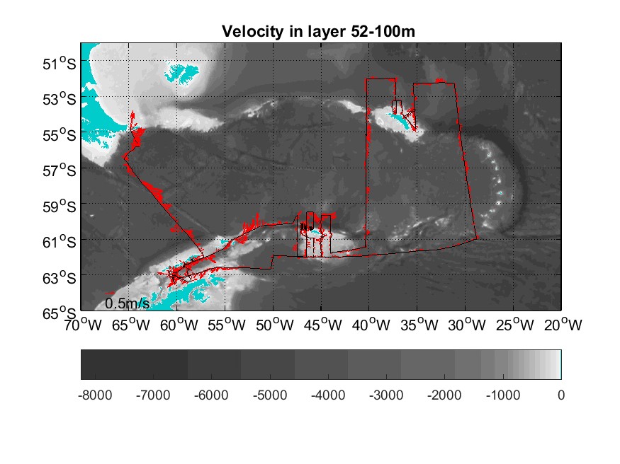
Current speed and direction measurements (ADCP)
Two drop keel mounted Acoustic Doppler Current Profiler (VMADCP) from RD Instruments ran during the survey. The frequency of the VMADCP are 38 and 150 kHz. The ADCPs were run in narrow band mode and set to estimate the current in 24 and 8 m vertical bins at 38 and 150 kHz. To prevent interference with the SIMRAD EK80 echosounder, both ADCPs and the echosounder was set up to ping at predetermined interval at signals from the SIMRAD K-sync system.
The 38 kHz perform very well, giving data down to at least 900 m in deep water, and 1450 m in favorable conditions. The range of the 150 kHz was typically 200-250 m at the start of the cruise and the quality was worsening during the cruise. Closer inspection revealed that two of the beams were not performing and quality is thus substandard. We will thus only use the data from the 38 kHz ADCP.
The heading data to convert the current recorded in the ship-referenced coordinates to the absolute zonal and meridional components were obtained from the vessel’s differential GPS system, Seapath. The data were collected with the RDI VmDAS software and the ENR single ping data were processed and edited using the CODAS system (University of Hawaii).
Figure 7.2 Along track 38 kHz ADCP measured currents in depth range 52-100 m.
8 - CTD data
A total of 48 CTD stations were occupied during the cruise. CTD stations 3-39 and 42-43 were done using the big 24 bottle rosette from the main hangar. Due to winch issues, stations 40-41 and 44-51 were done using the small 12 bottle rosette from the CTD hangar. Sensors mounted on the Seabird 9/11 plus CTD package or included in the data stream included:
SBE 3P Temperature sensor, s/n 03-6275 (primary)
SBE 4C Conductivity sensor, s/n 04-4726 (primary)
SBE 5T submersible pump, s/n 05-9378 (primary)
Digiquartz Temperature Compensated Pressure Sensor, s/n 141612
Two RD Instrument LADCPs and an external battery package were mounted on the 24 bottle rosette.
Further information on sensor configuration, maintenance and calibration can be obtained from the IMR instrument engineers Asgeir Steinsland and Roy Robertsen.
The CTD was controlled by the instrument engineers through SBE Seasave software, version 7.26. GPS data (NMEA string) from the ship’s navigation system was logged with every scan for later LADCP processing.
During a CTD cast, the CTD package was lowered to 10 m for a 1-minute soak before bringing it back to the surface and subsequently lowering to the bottom/maximum depth (=1000 m). Niskin bottles were fired on the up cast after a 1-minute stop at the desired bottle depth. On stations with adverse weather conditions, the 5 m bottle was fired “on the fly” to avoid strain on the CTD cable.
During CTD station 3 (the first of this cruise), the SBE Microcats that were later deployed on the moorings near Deception were tied to the CTD rosette frame for a calibration cast.
CTD station 7 was run for a sampling experiment for eDNA and therefore went only to 30 m depth with extended time between bottle firings.
Issues with the winch system in the main hangar led to the CTD being stopped for an extended period on a few casts, and in particular during cast 39. Repeated issues with the winch system required change over to the small CTD in the CTD hangar for CTD station 40. The entire CTD sensor package was moved and mounted on the small rosette frame by the instrument engineers which took about an hour. After CTD station 41, it was decided to try to use the big rosette again, but continuing problems led to the final switch back to the small rosette after CTD station 42.
All CTD sensors worked well throughout the cruise and no sensor failures occurred. Niskin bottles leakages were reported after each station and handled by the instrument engineers. After longer periods of the bottles being exposed to cold temperatures in the main hangar (as the main roll gate to the hangar got damaged during passage, it could not be closed completely) in cocked position leaving the rubber bands extended, leakage was considerable and the rubber bands had to be tightened accordingly.
Table 8.1. List over all CTD stations
CTD st #
P #
Year
Mon
Day
Hr
Min
Lat Deg [S]
Lat Min
Lon Deg [W]
Lon Min
Echo depth [m]
number of salt samples
LADCP yes/no
3
P54
2019
1
17
12
20
62
15.60
58
19.80
558
4x2 for testing
(y)
4
P02
2019
1
18
8
30
62
44.63
60
49.97
558
5
n
5
P55
2019
1
18
14
23
63
9.72
60
28.47
670
3
y
6
P01
2019
1
18
22
7
63
28.54
60
12.23
121
3
n
7
M3
2019
1
19
4
12
62
58.70
60
28.27
231
-
n
8
M5
2019
1
19
10
30
63
0.28
60
24.84
587
3
y
9
M7
2019
1
19
16
12
63
0.95
60
20.69
763
3
y
10
P04
2019
1
20
1
31
63
20.39
58
33.11
61
1
y
11
P56
2019
1
20
7
15
62
46.66
58
51.97
1335
-
y
12
P03
2019
1
20
19
36
62
30.60
59
18.56
602
3
y
13
P05
2019
1
22
15
44
59
39.99
47
30.01
4000
4
(y)
14
P06
2019
1
23
0
3
60
4.81
47
30.09
2009
4
y
15
P07
2019
1
23
4
38
60
29.98
47
30.02
805
3
y
16
P08
2019
1
23
10
5
60
55.18
47
29.93
2000
-
y
17
P09
2019
1
23
15
43
61
19.79
47
30.03
2747
4
y
18
P10
2019
1
24
5
44
61
19.79
46
29.94
316
1
n
19
P11
2019
1
24
10
38
60
55.21
46
30.10
333
4
n
20
P12
2019
1
24
16
38
60
22.48
46
30.01
923
4
y
21
P13
2019
1
25
2
15
60
4.79
46
29.85
2426
1
y
22
P14
2019
1
25
8
5
59
40.34
46
30.11
3402
-
y
23
P15
2019
1
25
16
23
59
40.21
45
44.98
2179
4x6 for testing
y
24
P16
2019
1
25
22
0
60
4.70
45
45.05
4809
3
y
25
P17
2019
1
26
3
48
60
25.78
45
45.07
293
1
y
26
P18
2019
1
27
18
54
60
55.23
45
44.99
245
1
n
27
P20
2019
1
28
3
14
61
45.01
45
44.89
393
3
y
28
P21
2019
1
28
11
57
61
44.87
45
0.11
376
1
y
29
P23
2019
1
29
2
14
60
55.21
44
59.96
236
4
n
30
P24
2019
1
29
8
1
60
29.98
44
59.91
370
-
y
31
P25
2019
1
29
13
7
60
4.78
44
59.83
5187
5
y
32
P26
2019
1
30
0
28
59
39.98
44
59.87
2755
5
y
33
P29
2019
1
30
14
15
60
29.97
44
0.08
2000
3
y
34
P30
2019
1
30
19
57
60
55.17
44
0.02
254
4
y
35
P32
2019
1
31
4
45
61
44.96
44
0.01
695
4
y
36
P33
2019
1
31
18
26
61
26.38
40
20.49
3496
5
y
37
P34
2019
2
1
13
59
59
32.34
40
19.62
2010
4
y
38
P35
2019
2
2
2
1
58
4.15
40
18.20
3290
5
y
39
P36
2019
2
2
13
60
56
32.27
40
18.39
3500
4
y
40
P37
2019
2
3
1
57
55
8.30
40
16.87
3731
4
n
41
P38
2019
2
3
13
59
54
38.15
40
15.77
3500
5
n
42
P39
2019
2
4
2
0
53
17.00
40
16.26
2917
5
y
43
P40
2019
2
4
14
7
52
0.54
40
8.55
3651
4
y
44
P51
2019
2
11
21
21
60
58.99
28
44.75
4220
6
n
45
P59
2019
2
14
19
1
62
0.94
50
0.44
3304
5
n
46
M9
2019
2
17
1
34
63
9.53
59
50.49
343
4
n
47
Mx
2019
2
17
3
4
63
5.78
60
3.90
835
4
n
48
M8
2019
2
17
4
47
63
1.80
60
17.61
849
4
n
49
M7
2019
2
17
5
58
63
1.01
60
21.13
724
3
n
50
M5
2019
2
17
7
10
63
0.06
60
24.82
581
4
n
51
M3
2019
2
17
8
32
62
58.83
60
27.79
373
4
n
Data processing
IMR routines
The Seasave software saves a suite of files for each cast with the following appendices: .XMLCON – instrument configuration file; .hdr – information header for each cast; .hex – the data file in binary format; .bl and .ros – information on the bottle firings of the rosette.
Initial CTD data processing was done according to standard IMR procedures using the SBE Data Processing software Version 7.26. The routines employed were:
datcnv
wildedit
celltm
filter
loopedit
derive
binavg
The resulting data files will be stored at the National Marine Datacentre at IMR.
Matlab-based postprocessing
For research purposes, CTD data were also processed using a suite of Matlab routines after an initial pass through selected SBE routines. Raw binary data were converted to ASCII using datcnv. Align CTD was applied to temporally align the CTD readings. CellTM was used to correct for the thermal mass of the cell. The resulting .cnv file was then treated in Matlab:
ctdcal.m: reads in the .cnv file
offpress.m: apply a pressure offset for each cast. This was typically between 0-0.6db.
spike_t90.m: remove large single point spikes
wake.m: remove wake which occur e.g. due to rolling of the ship
interpol.m: interpolate across NaNs to create a continuous data set
makebot_t90.m: read in bottle files created by Seasoft and extract CTD data during bottle firings
getsalts_t90.m: add bottle sample salinity where available and calculate offsets between CTD and bottle salinities
setsalflag.m: flag bottle salinities that should be discarded
salplot.m: plot to check bottle vs CTD salinities for further QC
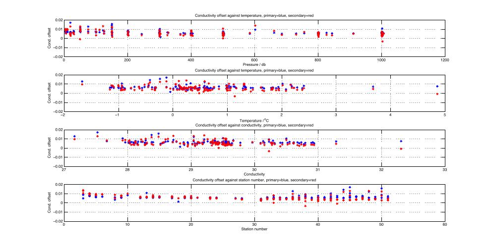
condanalyse.m: plot the conductivity offsets for all bottle firings against various variables and calculate the median conductivity offset for each sensor
saloffset.m: apply conductivity calibrations and calculate salinity and potential temperature
oxyoffset.m: apply oxygen calibration
splitcast.m: split the cast into up- and downcast
ctd2db.m: bin the CTD downcast data in 1 decibar bins
repeat makebot_t90.m, getsalts_t90.m and setsalflag.m to produce bottle files with calibrated conductivity and salinity.
For detailed information on the Matlab routines, see the JC087 CTD processing report produced by Gilian Damerell at UEA, UK. The routine for the oxygen calibration was added by A. Renner based on a routine written by Andrew Thompson for JR158 (ADELIE) in 2007 (see their cruise report).
The resulting Matlab-files were then written out as ASCII-files and made available to all cruise participants.
Salinity calibration
A total of 178 water samples were taken from selected depths after most CTD casts for calibration of the conductivity sensors and testing of the new salinometer (see Table 8.1). 250 ml flat bottles and their caps were rinsed three times with water from the CTD Niskin bottles before filling to just under the shoulder. The necks and caps were wiped dry to prevent any salt cristallisation which could contaminate the sample. Bottles were then sealed with single use plastic insert and the original bottle caps.
A new salinometer was purchased for use onboard the Kronprins Haakon. The Optimare Precision Salinometer (s/n 018) was first tested during the Fram Strait cruise in 2018 and a faulty heating element for the pre-bath required repair at the manufacturers. This cruise was the first to use the instrument after the repairs. After a few measurement runs with test samples tapped from the underway system, it quickly became clear that the heating element was again faulty. Through email discussions with the manufacturers and further extensive testing, including comparison to measurements using a Guildline Portasal (s/n 66999), a setup was found that allowed for stable measurements: Settings of the pre-bath stirrer and cooler were changed to manual control and set to minimise temperature changes (stirrer at approx.. -30 to -40, cooler to approx. 8), allowing instead for the pre-bath to adjust to surrounding temperatures. Instead of relying on preheating of the sample to the desired temperature during passage through the pre-bath, the residence time in the main bath was extended to the maximum allowed time (120 s) which allowed the conductivity reading to stabilise. This considerably prolonged the time required for sample processing. However, the stable readings and otherwise automated measurements were found superior to the Portasal procedures.
The Optimare salinometer is more sensitive to gas bubbles in the samples than the Portasal. Samples were therefore treated according to the Optimare manual: After a crate was filled and placed in the salt lab, the sample bottle were shaken and placed in a lukewarm water bath. After the bath had cooled down to room temperature, the bottles were shaken again, and pressure released by opening the bottles. Care was taken not to contaminate the samples with water droplets or damage the plastic insert before resealing the bottles. Samples were then left for at least one day before shaking them again and measuring.
Before each measurement session, standardisation was performed using OSIL IAPSO standard seawater (batch 151, K15=0.99987, S=34.995). On some occasions, near surface samples contained high plankton concentrations which could affect the conductivity cell in the salinometer. When this was the case, conductivity readings would typically show high drift or unstable readings. These samples were discarded, and the conductivity cell cleaned with bleach and Triton-X following the instructions in the Optimare manual before continuing with measurements.
Comparison of the bottle salinities and the CTD salinities using the above described Matlab routines showed that the CTD salinities/conductivities were too high compared to the water samples (see Figure 8.1). The primary conductivity sensor was stable throughout the cruise whereas the secondary sensor shows signs of drift. The primary sensor was therefore used to produce the final data files. The offset applied to either sensor (i.e. subtracted from the CTD values) was:
cond1: 0.0058526
cond2: 0.0050217
Figure 8.1. Comparison of conductivity offset against pressure, temperature, conductivity, and station number (from top to bottom) for primary and secondary conductivity sensor (blue and red, respectively).
In addition to the water samples from the Niskin bottles, 22 samples were taken throughout the cruise from the underway system for calibration of the thermosalinograph which continuously monitors water properties from the seawater intake. The samples were taken and treated in the same way as the CTD samples.
Oxygen calibration
Samples were taken for calibration of the dissolved oxygen sensor on the CTD. For a description of the Winkler titration method and the bottle results.
Figure 8.2 shows a comparison of the CTD to the Winkler values. The samples from CTD station 39 are clear outliers and were not included in calculation of the regression.
Using linear least squares regression yields the following relationship between Winkler and CTD derived oxygen concentrations [ml/l]:
Winkler O2 = -0.128465 + 1.009174 * CTD O2
with an R2 value of 0.973.
Figure 8.2. Comparison of Winkler-derived versus CTD-measured oxygen concentrations. Colours indicate CTD station numbers. The black line shows the result of the linear regression.
The equation was applied to the oxygen concentration in ml/l, and calibrated oxygen saturation and concentration in [μmol/kg] were derived in the final CTD processing.
Calibration of other sensors
Water samples for Chl a analysis were taken at all stations from bottles fired in depths >= 200 m. The filters will be analysed during the next cruise leg, and calibration of the CTD fluorescence will take place on land.
Preliminary results
The following figures show preliminary results from the main transect lines covered during the cruise and the stations around the South Orkney Plateau.
Figure 8.3. Potential temperature - practical salinity diagram of all CTD stations on the South Orkney Plateau and stations in the Weddell Sea (CTD stations 13-36, 44, 45).
Figure 8.4. Transect west of the South Orkney Plateau (CTD stations 13-17).
Figure 8.5. Transect across the Scotia Sea (CTD stations 36-43).
Figure 8.6. Transect along the mooring line near Deception Island, Bransfield Strait (CTD stations 46-51).
CTD data from krill trawl deployments
A SBE 37 Microcat was mounted on the krill trawl to collect temperature, conductivity and depth data during the trawls. The Microcat ran continuously from the first to the last trawl, and data were downloaded occasionally in between and after trawling was finished. Processing and calibration against the ship CTD will take place at IMR after the cruise.
9 - Chemical indicators to monitor Ocean Acidification
The main objective was to investigate the ocean acidification state and carbon cycling across contrasting oceanographic and biological regimes of coastal Antarctic waters and the Southern Ocean. More specifically, we aim at improving the understanding of the feedbacks by physical and biogeochemical processes in the regions of active krill fisheries, with respect to the distribution of the carbonate chemistry, air-sea CO2 fluxes and transport of anthropogenic CO2.
Work at sea
We sampled seawater for the four core carbonate system parameters: dissolved inorganic carbon (DIC), total alkalinity (TA), pH, and the partial pressure of CO2 (pCO2) and stable oxygen isotope (δ18O). Two of these will be used to derive all other carbonate chemistry parameters such as CaCO3 saturation and aqueous CO2. Seawater samples were taken from the Niskin bottles mounted to the large and small CTD-rosette from 12-15 depths throughout the water column. A total of 45 stations, comprising 1239 sample analyses taken for carbonate chemistry analysis (onboard) and 479 taken for δ18O storage (cool fridge) and post-cruise analysis. Table 9.1 summarizes the sampling from the water column using the CTD-Rosette and Figures 9.1 and 9.2 show preliminary data.
Carbonate chemistry and δ18O isotope
The samples for carbonate chemistry were taken first, or directly after dissolved oxygen samples when taken, and analysed within 24-hours for the determination of pH, total inorganic carbon (DIC) and total alkalinity (AT). Samples were taken into borosilicate bottles (250 mL), with tight plastic screw caps, and were rinsed with at least one bottle volume and filled to the rim. All samples were thermostated to 20°C prior to analysis.
Seawater pH was determined spectrophotometrically (Clayton and Byrne, 1993) using the sulfonephthalein indicator m-Cresol Purple (mCP). The indicator solution (0.2 mM) was prepared by dissolving pre-weighed mCP indicator in 0.5 L filtered seawater (0.20 µm) of about salinity 35. The indicator was adjusted to a pH in the same range as the samples, approximately ± 0.2 pH units, by adding a small volume of concentrated HCl or NaOH. During each analysis period (within 24-hours) the pH of the indicator was measured using a 0.02 cm cuvette. The magnitude of the perturbation of seawater pH caused by the addition of indicator solution is calculated and corrected for using the method described in Chierici et al. (1999). The instrument setup is controlled by a PC running a LabView program (Fransson et al., 2013). The pH values are corrected to 25°C on the total scale. The overall precision from duplicate sample analysis was better than ±0.001 pH units. The accuracy was checked against Certified Reference Material for total alkalinity and total dissolved inorganic carbon, indicating that it should be well below 0.01 pH units.
The concentration of DIC, the sum of all dissolved inorganic carbon species, was determined by a coulometric method (Dickson et al., 2007) using a VINDTA 3D instrument (MARIANDA, Kiel). The TA analysis were made by potentiometric titration with HCl as a titrant. The acid consumption up to the second endpoint is equivalent to the titration/total alkalinity. The system uses a precise Metrohm Titrino, a pH electrode and a reference electrode. The accuracy for DIC and TA analysis is set by internationally recognized certified reference material (CRM, batch 173) obtained from Prof. A. Dickson at Scripps Institute of Oceanography (USA). One CRM was analysed in duplicate at the beginning of the DIC and TA analyses. The precision for DIC and TA was determined from the in-bottle CRM duplicate analyses to be better than 2 µmol/kg. The accuracy was checked against frequent analysis of CRMs.
Surface water oxygen, CO2 and air-sea CO2 exchange
Surface water partial pressure of CO2 (pCO2) was determined along the cruise track from the ship’s underway seawater supply. Sea surface pCO2 is obtained with a General Oceanics (GO850) system with an infra-red analyser (LiCOR 7000), alongside dissolved oxygen (Aanderaa sensor). Air-sea fluxes will be determined from the gradient of pCO2 in air and seawater and wind speed. Underway samples were taken throughout the cruise to check the instrumentation and the performance.
Table 9.1. Seawater samples taken from CTD-Niskin rosette system for each station.
year
month
day
latitude
longitude
station
CTD
pH
DIC
TA
δ18O
2019
1
17
-60,2600
-58,3300
P54
3
x
x
x
x
2019
1
18
-62,7438
-60,8328
P2
4
x
x
x
x
2019
1
18
-63,1620
-60,4745
P55
5
x
x
x
x
2019
1
18
-63,4757
-60,2038
P1
6
x
x
x
x
2019
1
19
-63,0047
-60,4140
8
x
x
x
x
2019
1
19
-63,0158
-60,3448
9
x
x
x
x
2019
1
20
-63,3398
-58,5518
P4
10
x
x
x
x
2019
1
20
-62,7777
-58,8662
11
x
x
x
x
2019
1
20
-62,5100
-59,3093
12
x
x
x
x
2019
1
22
-59,6665
-47,5002
P5
13
x
x
x
x
2019
1
23
-60,0802
-47,5015
P6
14
x
x
x
x
2019
1
23
-60,9197
-47,4988
16
x
x
x
x
2019
1
23
-61,3298
-47,5005
P9
17
x
x
x
x
2019
1
24
-60,9202
-46,5017
19
x
x
x
x
2019
1
24
-60,3747
-46,5002
P12
20
x
x
x
x
2019
1
25
-60,0798
-46,4975
P13
21
x
x
x
x
2019
1
25
-59,6723
-46,5018
22
x
x
x
x
2019
1
25
-59,6702
-45,7497
P15
23
x
x
x
x
2019
1
25
-60,0783
-45,7508
P16
24
x
x
x
x
2019
1
26
-60,4297
-45,7512
P17
25
x
x
x
x
2019
1
27
-60,9205
-45,7498
26
x
x
x
x
2019
1
28
-61,7502
-45,7482
P20
27
x
x
x
x
2019
1
28
-61,7478
-45,0018
P21
28
x
2019
1
29
-60,9202
-44,9993
P23
29
x
x
x
x
2019
1
29
-60,4997
-44,9985
30
x
x
x
x
2019
1
29
-60,0797
-44,9972
31
x
x
x
x
2019
1
30
-59,6663
-44,9978
P26
32
x
x
x
x
2019
1
30
-60,4995
-44,0013
P29
33
x
x
x
x
2019
1
30
-60,9195
-44,0003
34
x
x
x
x
2019
1
31
-61,4397
-40,3415
P33
36
x
x
x
2019
2
1
-59,5390
-40,3270
P34
37
x
x
x
x
2019
2
2
-58,0692
-40,3033
38
x
x
x
x
2019
2
2
-56,5378
-40,3065
P36
39
x
x
x
x
2019
2
3
-55,1383
-40,2812
40
x
x
x
x
2019
2
3
-54,6358
-40,2628
P38
41
x
x
x
x
2019
2
4
-53,2833
-40,2710
42
x
x
x
x
2019
2
4
-52,0090
-40,1425
P40
43
x
x
x
x
2019
2
14
-62,0157
-50,0073
P59
45
x
x
x
2019
2
17
-63,1588
-59,8415
46
x
x
x
2019
2
17
-63,0963
-60,0650
47
x
x
x
2019
2
17
-63,0300
-60,2935
48
x
x
x
2019
2
17
-63,0168
-60,3522
49
x
x
x
x
2019
2
17
-63,0010
-60,4137
50
x
x
x
x
2019
2
17
-62,9805
-60,4632
51
x
x
x
x
Preliminary results
Figure 9.1. Sea surface CO2 from the underway pCO2 instrument along the cruise track.
Figure 9.2. Sea surface DIC and profiles of DIC in the upper 1000 m as surveyed at all stations sampled (Table 9.1) during the cruise.
10 - Dissolved Oxygen
In order to calibrate the oxygen sensor and get accurate value of dissolved oxygen, we sampled seawater from Niskin bottles and the underway system.
Methods
We sampled seawater from Niskin bottles mounted onto a CTD-Rosette from 6 to 14 depths in the water column at 20 stations. A total of 243 CTD-Rosette seawater samples were analyzed.
We also sampled seawater from the underway system at 5 stations (25, 26, 28, 44, 45). The underway system is taking water at 4-meter depth every 2.5 minutes.
Oxygen titration
The oxygen was analyzed using the Winkler titration for all water samples. The method is based on the classical Winkler method with respect to sampling and reagents up to the point of titration with thiosulfate, according to the following redox-reactions:
First an excess of dissolved manganese and a strong base with an excess of iodide ions are added to the seawater sample, the Mn2+ is oxidized by the dissolved oxygen in the water to higher oxidation states and precipitates as MnO(OH)2 to the bottom of the sample bottle. After a few hours, an excess of strong acid is added to the sample, to reduce the manganese back to the Mn2+ form. With the reduction of manganese, the iodide ions become oxidized to iodine in the form of I3- ions, which has an intense yellow colour. And this was titrated with sodium thiosulfate.
Results
Table 10.1. Mean difference between oxygen values estimated by the Winkler titration and by the oxygen sensor mounted on the CTD-Rosette.
Station number
Station name
Number of sample
Mean difference (ml/L)
Underway system difference (ml/L)
3
P54
14
0.2006
4
P02
6
-0.1924
6
P01
7
0.3141
8
M5
11
0.3029
9
M7
8
0.2468
12
P03
12
0.1498
13
P05
11
0.0751
17
P09
12
0.1055
20
P12F
13
0.1931
25
P17
13
-0.1690
-4.0847
26
P18
8
0.0555
-3.8553
28
P21
10
0.0574
-3.7962
30
P26
11
-0.2572
31
P27
7
-0.1682
33
P29
11
-0.0679
36
P33
9
0.1578
37
P34
10
-0.4243
41
P38
11
-0.0685
43
P40
10
0.0877
44
P51
12
0.1766
-3.3752
45
P59
12
0.2459
-3.7307
49
M7
10
0.3645
Mean
10.4
0.2623
-3.55295
10.2.1 - Preliminary results
The mean difference between the underway system sensor and the Winkler titration is -3.55295 ml/L. To have comparable results, the mean difference was subtracted from the oxygen values given by the underway system sensor. The same calculation was applied to the CTD values.
Figure 10.1. Map of the surface oxygen estimated by the underway-system
Figure 10.2. Map of the surface oxygen estimated by the CTD
11 - Sailbuoy with acoustics
This measurement trial consists of an autonomous measurement platform using acoustic measurements to measure krill. The measurement platform is the wind driven ASV Sailbuoy, developed by Christian Michelsen Research, and commercialized by Offshore Sensing AS. Since it is wind-driven has low self-noise, which makes it well suited for acoustic measurements. The sampling scheme is selected to ensure that the battery will keep a full charge for the measurement period. The main specifications of the Sailbuoy is given in Table 11.1.
Table 11.1. Sailbuoy specifications.
Length
2 m
Height
1.5 m
Weight
60 kg
Payload capacity
10 kg
Speed
1-3 knots
Operational duration
< 1 year
Communication
Iridium satellite link
The Sailbuoy is equipped with a Simrad EK80 broadband echosounder, with a 200 kHz transducer mounted in the keel. The transducer is mounted in a gimbal to reduce the effect of roll on the acoustic measurements. A web server is used for communication with the Sailbuoy, and for giving waypoints for it to follow. The control and communication with the Sailbuoy go through an Iridium satellite link. The Sailbuoy and echosounder mounted in the keel is seen in Figure 11.1.
Figure 11.1. The Sailbuoy autonomous surface vehicle (left) and the transducer mounted in a gimbal in the keel (right).
A crane with quick release was used to deploy the Sailbuoy, and it was recovered using crane with a rope around the sail and mast.
Results
The deployment period of the Sailbouy was from January 19 to February 16 and within the area of Branfield Strait. During this time, it sailed approx. 1200 nautical miles. The echosounder collected data with a duty cycle of approx. 20 %. In addition to active ping mode, passive pings were used in order to estimate noise. The measurement range of the transducer was 300 m. The Sailbuoy track plan was to overlap with the transect of the acoustic moorings deployed on this cruise, in addition to cover the transect in Bransfield Strait defined by the two coordinates in Table 11.2.
Table 11.2. Transect details.
Code
Lat
Lon
AP15_north
-63.34
-58.55
AP15_south
-62.51
-59.31
During the deployment, valuable information was gained about the Sailbouy navigation regarding different wind conditions in the Antarctic waters.
Figure 11.2. The track of the ASV during the measurement period. The Sailbuoy covered approx. 1200 nautical miles.
The acoustic results of the ASV survey will be processed after the cruise. Some preliminary goals for data processing include
Comparison with acoustic data from moored echosounders
Krill biomass estimation, comparison with RV Kronprins Haakon acoustic measurement
12 - LADCP measurements
Two RD Instruments 300 kHz Workhorse ADCPs were mounted on the 24-bottle CTD rosette with a shared external battery pack (s/n 24472 looking upward; s/n 24474 looking downward). The ADCPs were started and stopped using BBTalk on a laptop in the fine electronics workshop before and after each cast. For an overview of CTD stations during which LADCP data were collected see Table in CTD report. During CTD station 3, a test profile was collected. During CTD station 13, the protective caps were not removed rendering the profile unusable.
The LADCPs were set up with the downward looker as master and the upward looker as slave. The following configurations were used:
15 bins with 8 m bin depth, 2.5 m s-1 ambiguity velocity, automatic ping cycling, narrowband
Data processing
Data was downloaded by the instrument engineers after each cast and checked periodically using WinADCP software. Processing will take place on land using the latest available version of the LDEO LADCP processing routines.
13 - Krill sound speed and density contrast
The contrast between sound speed and density of Antarctic krill and seawater was measured using the APOP (Acoustic Properties Of zooPlankton) technique (Chu et al., 2000; Chu and Wiebe, 2005). The sound speed was inferred from the time difference for an acoustic pulse to travel through seawater and then through a mixture of krill and seawater (Figure 13.1). The density and volume of krill was inferred using a dual-density method, via measurements of the weight of the krill & some seawater, the weight of krill, seawater, and fresh water of a known volume, and measurements of the densities of the freshwater, seawater, and mixture of seawater and freshwater.
The sound speed measurements were taken in a bath of seawater at a temperature of between 3 and 16 °C. Temperature and salinity were measured and recorded every 2 seconds using an Aandreaa 4119 conductivity/temperature sensor, which also provided sound speed estimates. An acoustic pulse of 500 kHz and 5 cycles duration was transmitted through the animal chamber and received with by a PicoScope PC-based oscilloscope. The average received signal from 300 pings (at 5 Hz ping rate) was recorded for transmission through seawater and then repeated with about 15 krill inserted into the animal chamber.
Weights were taken using a pair of Kern ALJ 250-4AM balances that output instantaneous weight measurements at 5 Hz rate to a nominal precision of 0.1mg. One balance always had a nominal 50 g weight on it, while the other held the object being weighed. Custom-written software calculated the object weight by reference to the value from the balance holding the 50 g weight. At least 10 000 readings were taken for each weighing operation and the average taken to estimate the object weight. The density of the freshwater, seawater, and mixed water was measured using an Anton Paar 4500M density meter with a nominal accuracy of 10-5 g cm-3. The weights and density measurements were taken at ambient temperature, nominally 20°C.
A sample (10-20 individuals) of live or freshly dead krill were measured from all trawls that caught enough krill. For selected trawls, three separate measurements were made per trawl to evaluate the variability within a trawl catch.
Figure 13.1. Krill being placed into the submerged sound speed measuring chamber (left image); krill in the container ready for weighing.
Results
Measurements were taken from 26 trawls. For 6 of these trawls, triple measurements were made, for a total of 37 sound speed and density measurements throughout the survey area, except for Bransfield Strait were no measurements were made.
These experiments were funded by a grant from the Antarctic Wildlife Research Fund to the Australian Antarctic Division (AAD) in collaboration with IMR, NOAA (USA), and the YSFRI (China).
Two sets of APOP equipment were constructed – the second was onboard Cabo de Hornos, which conducted most of the 2019 krill acoustic survey. Analysis and reporting will be carried out by the project partners and presented at the June 2019 CCAMLR SG-ASAM meeting.
14 - Acoustic backscatter of krill measured with lowered transducer
A scientific broadband echosounder equipped with custom-made, narrow beam-width transducer was used to measure individual krill as single objects/targets rather than schools (Figure 14.1). This is hard to achieve as krill tend to school in high density schools making it near impossible to measure single krill by ship-mounted echosounders. Goal was to measure broadband acoustic backscatter of individual krill to (i) test a concept of possible remote sizing of krill from broadband data, (ii) investigate acoustic frequency response of individual krill at 160-260kHz and (iii) measure acoustic target strength of krill in situ. Tight survey schedule did not allow for targeted measurements over selected krill swarms thus data were collected opportunistically during nocturnal CTD stations. Total of 16 one-two hour long drops were performed of which 4 drops contain useful data.
Figure 14.1. Simrad EK80 broadband echosounder transceiver coupled with custom-made 3° beam-width transducer (orange). Transducer equipped with 30m cable was suspended by rope over ship side to 15m depth. Transducer was mounted inside protective steel mount.
Material and methods
A Simrad EK80 broadband echosounder equipped with custom-made one-of-the-kind transducer ES-200-3C was used to obtain fine scale acoustic records of krill resolved as single objects/targets rather than schools/layers. Echosounder transducer was opportunistically deployed over ship side during some of the nocturnal CTD stations – the only time ship is stationary. Nocturnal observations were selected because krill tend to rise close to the sea surface and is thus more accessible for the fine-scale, close range acoustic measurements.
Echosounder was calibrated according to the standard methods (Demer et al., 2015) and using standard tungsten carbide calibration sphere (WC38.1). Echosounder calibration was performed with transducer suspended by crane over the side of the ship at 2m water depth. This was done just after the ship echosounder calibration exercise held on 2019.01.16 (Admiralty bay of King Georg I island, Bransfield Strait). Transducer was mounted in a specially made steel protective mounting (Figure 14.1). Transducer is equipped with 30m long cable which enabled data collection with transducer deployed to 15m water depth over the ship side at the mid-ships. Only dorsal aspect acoustic backscatter data were collected. Echosounder settings for data collection are listed in Table 14.1.
Table 14.1. Parameter settings of Simrad EK80 split-beam echosounders used. “c.f.” refers to values at “centre frequency”, i.e. 200kHz. Most of the acoustic data were collected using ‘fast’ power ramping setting.
Parameter
Transducer type
ES200-3C
Bandwidth [kHz]
160-260
Transmission power [W]
50
Filter slope, fast power ramping [%]
50
Filter slope, slow power ramping [%]
1.2
Nominal gain at c.f. [dB]
34.0
Nominal absorption coefficient at c.f. [dB]
42.8
Half-power beam widths (along-ship/athwartship) at c.f. [deg]
2.93/2.95
Pulse duration [ms]
1.024
Ping rate [s-1]
4-9
Sound speed [m/s]
1452.7
14.2 - Results
About 25 hours of broadband acoustic data were collected over 16 echosounder drops. All collected acoustic data is summarised in Table 14.2. Example echogram (Figure 14.2) demonstrates one of the best data samples obtained. It shows a krill school at 20m depth (5m below transducer). Individual krill can be resolved on the upper outskirts of the school. The line graph exemplifies acoustic frequency response over 160-260kHz band for 4 individual krill measured at the last ping of this echogram. The distinct pattern and “dips” in the frequency response graph may be associated with the physical dimensions of individual krill, i.e. krill size.
Figure 14.2. Example echogram from the lowered transducer data set No. 12. Krill swarm is observed at 20-25m under the ship (5-10m under the transducer). Vertical axis is 15m of range under the transducer. Horizontal axis is time (1.5min). Individual krill resolved as single tracks can be seem on the upper part of the school. Line graph demonstrates acoustic frequency response at 160-260kHz for 4 resolved individual krill at the last ping of the echogram.
Table 14.2. Brief summary of the collected broadband acoustic data.
ID
Date/start time (UTC)
Lat./Long.
Krill in data
Trawl sample
Drop-1
2019.01.28/03:19:50
-61.750 / -45.748
Krill
Yes
Drop-2
2019.01.29/02:18:30
-60.920 / -44.999
No krill
Yes
Drop-3
2019.01.30/00:34:28
-59.666 / -44.997
No krill
Yes
Drop-4
2019.01.30/20:06:03
-60.919 / -44.000
No krill
Yes
Drop-5
2019.01.31/04:51:13
-61.749 / -44.000
Krill
Yes
Drop-6
2019.02.02/02:10:45
-58.069 / -40.303
No krill
Yes
Drop-7
2019.02.02/14:10:35
-56.537 / -40.306
No krill
Yes
Drop-8
2019.02.03/02:01:55
-55.138 / -40.281
No krill
Yes
Drop-9
2019.02.11/20:05:47
-60.983 / -28.746
No krill
Yes
Drop-10
2019.02.11/21:25:27
-60.983 / -28.746
No krill
Yes
Drop-11
2019.02.14/19:02:48
-62.015 / -50.007
No krill
Yes
Drop-12
2019.02.17/01:39:41
-63.158 / -59.841
Krill
No
Drop-13
2019.02.17/03:11:16
-63.096 / -60.065
No krill
No
Drop-14
2019.02.17/04:52:47
-63.030 / -60.293
Krill
No
Drop-15
2019.02.17/06:02:50
-63.016 / -60.352
Krill
No
Drop-16
2019.01.17/07:14:01
-63.001 / -60.413
No krill
No
15 - Echosounder moorings
Nine acoustic/oceanographic moorings were deployed for the duration of the cruise in Bransfield Strait. Two of these were deployed adjacent to Nelson Island, while the remainder were deployed in a south easterly section from Deception Island. The moorings contained a mixture of instruments (Table 15.1, Figure 15.1): three were pure echosounder moorings (Simrad WBATs), three were Nortek Signature 100 ADCP/echosounders, and the remainder each held two Nortek Signature 250 current profilers (arranged as a upwards and a downwards-looking pair). Selected moorings also included Seabird SBE37 CTDs and one a SeapHOx pH sensor. Two of the Signature 100 moorings (1 & 9) were supplied by NOAA.
The WBAT’s operated at 70 kHz and were programmed to operate for 1 hour and 18 minutes every 2 hours and 20 minutes, pinging every 0.9 seconds, through to the 18th of February. The Signature 100’s produced three different pings (70, 120 kHz, and a 70-120 kHz chirp ping that was internally split into 5 frequencies centred on 73, 82, 90, 99, and 107 kHz). The Signature 100 pung every 6 seconds for the entire deployment period. The Signature 250’s recorded 4-minute averages every 10 minutes and the CTDs recorded data every 5 minutes or better.
The WBAT echosounders were calibrated as per normal procedures (Demer et al., 2015) while anchored in Admiralty Bay, King George Island on 16 February. The depth of the transducers during the calibration was approximately 2 m. A calibration at anticipated deployment depth was not attempted. The Signature 100’s were not calibrated during the voyage.
Moorings 1 & 2, 4 & 5, and 5 & 6 were placed adjacent to each other for comparison purposes (Figure 1.4).
Results
All mooring equipment operated generally as planned. The quality of the acoustic data was excellent with a good signal-to-noise ratio at the maximum range. Evidence of tilting and push down was evident in all moorings. For an unknown reason, the echosounder on mooring 1 stopped collecting data on the 13th of February. The acoustic release on mooring 6 did not respond to release commands and was trawled up without loss of, or damage to, the equipment.
The echosounders observed many krill schools and many instances of diving predators (Figure 15.2 and 15.3). The faster ping rate used on the WBAT’s gave echograms where it was much easier to see predators diving. In many cases the split-beam ability of the WBAT’s also provided good quality 3D positions of diving predators.
Analysis of these data will be carried out by NOAA and IMR. NOAA has also carried out three passes over the Deception Island mooring transect with an autonomous glider and the oceanographic data from these will be available for use by IMR:
Table 15.1. Overview of the echosounder mooring configuration and data collected.
Mooring id
1
2
3
4
5
6
7
8
9
Equipment
1 x Signature 100, 2 x CTD
1 x WBAT
1 x Signature 100
1 x WBAT
2 x Signature 250, 3 x CTD
1 x WBAT
2 x Signature 250, 4 x CTD
2 x Signature 250
1 x Signature 100 1 x CTD
ADCP/echosounder serial no.
101132
266747
100764
253129
10552 (up) 10562 (down)
253126
10221 (up) 10397 (down)
10557 (up) 10561 (down)
101134
CTD serial no. (deployment depth, m)
16244 (530) 16241 (335)
n/a
n/a
n/a
20349 (50) 20350 (150) 20351 (300)
n/a
20354 (30) 20252 (150) 16246 (300) 20253 (500)
n/a
16567 (335)
Deployment area
Nelson Island
Nelson Island
Deception Island
Deception Island
Deception Island
Deception Island
Deception Island
Deception Island
Deception Island
Deployment latitude
S62° 21.634’
S62° 21.4379’
S62° 58.8377’
S62° 59.8140’
S63° 00.0761’
S63° 1.1340’
S63° 00.9611’
S63° 01.8036’
S63° 09.5599’
Deployment longitude
W059° 11.4371’
W059° 11.1419’
W60° 27.8012’
W060° 24.4440’
W60° 24.7376’
W060° 21.5580’
W60° 20.9690
W60° 17.6268’
W059° 50.7128’
ADCP/echosounder depth (m)
324
356
345
338
150
334
150
150
335
Bottom depth (m)
545
588
380
571
590
746
750
847
347
Nominal operating frequencies (kHz)
70, 120, 70-120 chirp
70
70, 120, 70-120 chirp
70
250
70
250
250
70, 120, 70-120 chirp
Nominal transducer beamwidth (°)
10
18
10
18
n/a
7
n/a
n/a
10
No. pings collected (‘000s)
401
1261
433
1149
n/a
1190
n/a
n/a
400
Start time (UTC)
18/1/2019 00:29
18/1/2019 02:00
19/1/2019 06:29
19/1/2019 10:00
19/1/2019 09:32
19/1/2019 20:00
19/1/2019 15:30
19/1/2019 18:00
19/1/2019 20:18
End time (UTC)
13/2/2019 17:39
18/2/2019 10:38
16/1/201 22:01
16/2/2019 20:38
16/2/2019 19:33
17/2/2019 21:45
16/2/2019 16:03
16/2/2019 15:00
16/2/2019 11:12
Duration of operation (days)
26.3
31.4
28.6
28.4
28.5
29.1
28.0
27.9
27.6
Figure 15.1. Left: a Simrad WBAT echosounder mooring ready for deployment. The orange disc is the acoustic transducer, the yellow cylinder (mostly obscured) is the WBAT echosounder, the yellow eelipsod the flotation, and the white/silver tube an ARGOS tracker. Right: A Nortek Signature100 echosounder mooring ready for deployment. The echosounder transducer is the black disk to the left, and the yellow discs the ADCP transducers.
Figure 15.2. Example echogram from mooring 2 showing predators diving towards krill schools at 100-160 m depth. Bubbles are released during the predator’s ascent, leading to the echoes that slowly ascent from left to right.
Figure 15.3. Example from mooring 2 showing several dives by animals, some of which release bubbles on their ascent.
16 - Environmental toxicology
The aim of this cruise was to collect samples for quantitative toxicological analysis in biological- and environmental compartments. The study focuses on Antarctic krill (E. superba), salps (S. thompsoni), krill predatory fish and water. The samples were collected over a large area to look for spatial distribution of mercury (Hg), per- and polyfluoroalkyl substances (PFAS) and persistent organic pollutants (POPs). Krill predatory fish were selected to assess the potential biomagnification of these contaminants in parts of the Southern Ocean food web. Biological samples will later be analyzed for stable isotopes of carbon and nitrogen (13C and 15N) to assess the effect of carbon source and trophic position on contaminant levels respectively (Hobson & Welch, 1992; Post, 2002)..
Material and methods
Biological and environmental samples were taken from a total of 44 stations during the area 48 survey. Biological samples include krill (E. superba), 5 (five) species of pelagic fish; P. Antarctic, G. nicholsi, G. braueri, E. Antarctica, C. rastrospinosus and salps (S. thompsoni) as principle study organisms. 4 (Van Dyck et al.) species of zooplankton were also sampled, including krill (E. triachanta), two species of amphipods and one species of salps. All species sampled were present in larger quantities over a wide geographical range and represented the majority of trawl catches.
Biological samples
Biota were sampled for analysis of total mercury (TotHg), POPs and stable isotope analysis (SIA) of 13C and 15N. Krill were sampled, live/active krill preferred, and packed in aluminum foil and zip-lock bag then stored at -30ºC. Both Hg, SIA and POPs samples were stored in this manner. Hg samples will later be analyzed by thermal decomposition, amalgamation, and atomic absorption spectrophotometry, method outline by U.S. Environmental Protection Agency . POPs samples were in addition packed in two layers of alcohol-rinsed aluminum foil. Krill were measured from rostrum tip to end of telson to the nearest 0.5mm, weight to be taken individually back in the lab for higher precision. Fish were dissected, and samples of liver and muscle were taken and stored at -30ºC. Fish were measured from head to tail fin base to the nearest mm and weighed to the nearest 0.1g. All other species of zooplankton were collected in 15ml/50ml polypropylene sample tubes. They were counted and weighed to the nearest 0.1g.
Environmental samples
Environmental samples included water samples for total mercury (TotHg), PFAS and POPs. PFAS water samples were collected from carrousel mounted Niskin bottles (CTD rig) at 50m depth in 1000ml PP (polypropylene) bottles, packed in double zip-lock bags and stored in cooler at ~ -3ºC for later analysis on shore (Chiang, 2016). TotHg water samples were collected from the same Niskin bottle at 50m depth in 250ml in FLPE (fluorinated high-density polyethylene) bottles and stored in the same manner as PFAS samples (Braaten, 2015; UEPA, 2002). As FLPE bottles are coated with a fluorinated compound the samples were handled and stored separately with great precaution. POPs water samples were collected with an AQUA-filter active pump unit, constructed at the University of Oslo on the design of a similar device used at NIVA (Norwegian Institute for Water Research). The AQUA-filter actively pumps water through one 293 mm glass fiber filter and two polyurethane filters (PUFs), with a flow-meter measuring water volume. The pump was lowered to 50m and started pumping after a set time delay. Filters were removed, packed in aluminum foil and stored at -30ºC for later analysis on shore.
Dataset
Table 16.1. Overview of sample dataset
Sample
Stations sampled
Number of samples
Locations sampled
Antarctic krill (E. superba)
24
408
Br, SO, SG
Hg/SIA
24
211
Br, SO, SG
POPs
18
197
Br, SO, SG
Fish (P. Antarctic, G. nicholsi, G. braueri, E. antarcitca, C. rastrospinosus)
5
36
Br, SO, SG
Salps (S. thompsoni)
7
7*
SO, SG
Water
31
31
Br, SO, SG
Hg
31
31
Br, SO, SG
PFAS
31
31
Br, SO, SG
POPs
1
1
SO
Zooplankton
3
5*
Br, SG
Total stations
44
*Pooled sample SIA = Stable Isotope Analysis Br = Bransfield strait SO = South Orkneys SG = South Georgia
17 - eDNAsampling
Studies of the distribution and abundances of Antarctic marine species arelimited by logistic challenges and costs associated with sampling.Although significant efforts are undertaken to assess Antarctic marine resources, the spatiotemporal assessment resolution is coarse, and changes in species’ spatiotemporal distributions may gounnoticed. Thorough surveillance by traditional approaches involved eployment of heavy gear and considerable efforts to process thecollected material. Increasing surveillance by methodologies that require less effort on the vessel may allow additional samplingplatforms (e.g. fishing vessels) to be employed and may thusre present a remedy to the problem.
A methodology that may meet the needs required for more comprehensive sampling in time and space is use of eDNA (environmental DNA) to detect presence of species. This methodology relies on molecular identification of trace amounts of shed DNA present in the environment to indicate presence and possibly abundance of a species (Klymus et al 2017, Yamamoto et al 2016). The only samples required are water samples from the CTD rosette that must be filtered either insitu or onboard using e.g. vacuum pump and filters. The methodology has successfully been used to qualitatively, and in some instances also quantitatively, demonstrate presence of species in a system. Use of eDNA may also be used to improve taxonomic resolution compared tothat usually obtained from sample processing.
eDNA approaches applies methodology from molecular biology (sequencing,qPCR, PCR, ddPCR, hybridization) to DNA-samples obtained from the environment. The presence and quantity of the DNA will depend on hydrography, location of the shedding source, and rate of degradation. These are all ecosystem-specific factors (e.g. Yamamotoet al 2016). The results will further depend on the sensitivity and accuracy of the analyses applied. The sensitivity and accuracy of the analyses, if a PCR based method is chosen, can be established in the laboratory using appropriate stored samples. However, effects of the remaining factors require carefully matched conventional and eDNAsamples. Such samples were obtained during the cruise (See table 17.1).
Materials and Methods:
Prevention contamination from equipment:
Beforesampling began the equipment to be used – including Niskin waterbottles - was washed in a 1% chlorine solution for minimum 30 minutes (based on Greenstone etal.2012). Commercial household bleach is typically 2-5% and was dilutedaccordingly (i.e. in the range from 1:2 to 1:5).
Watersampling:
When arriving at station CTD was run first to avoid contamination from other equipment that has been in the water (such as trawls) and to avoid aerosols. Niskin bottles were decontaminated with chlorine prior to station arrival. The CTD with Niskin bottle rosette is run down to the predetermined depths and the bottles are shot off (filled). Three Niskin bottles were released at each depth at allstations, except when winch faults prevented operation of the 24-bottle rosette forcing a single bottle pr. depth regime to beenforced when using the 12-bottle rosette.
Samplecollection from CTD:
When CTD arrived at deck water nozzles were treated with 1% bleach, left for 1-2 minutes and flushed with Milli-Q water. Two to five liters of water from each Niskin bottle (depending on whether the 12or 24 bottle rosette was used) were tapped onto bottles sterilized with 1% bleach. Bottle origin was noted to allow identification of possible “bottle effects”.
Filtrationof water:
Before filtering the tubes to be used, stored with 1% bleach when not in use, were flushed with minimum 250 ml Milli-Q water to remove bleach. Subsequently tubes were then flushed again with at least 250 ml ofthe water to be filtered prior to fitting of the filter cartridges.Filtration was performed by filtering 1 liter of water pumped at a flowrate of 100ml-min using a peristaltic pump through 0,22 µm Sterivex cartridge filters (Figure 17.1). After filtration the filters were dried by forcing 50 mlof air through them using sterile 50 ml syringes. The filters were then deposited in 50 ml centrifuge tubes and immediately frozen at -80 °C. Syringes were reused after sterilization by rinsing forminimum 30 minutes in 1% bleach.
Negative Air Controls were obtained by forcing 50ml air from a syringe through a filter. Two Negative Water Controls were obtained by pumping 1 l of Milli-Q water through filter. From each depth three replicate samplesfrom separate Niskin water bottles were filtered as described above. At the 2 stations (P37, P59) the 12-bottle water bottle rosette wasused, and replicates samples originated from the same water bottle. At these stations the tubes were not cleaned between replicates from the same depth.
Figure 17.1. Left: Sterivex filters during filtration – the leftmost filterfiltering water from 30 meters containing far more plankton than thedeeper samples to the right (100m. and 200m. respectively).
Establishingsignal variability baselines:
To investigate the potential effect of the time the samples spends on deck before it is filtered we constructed a set of samples that aged onboard. The sample was constructed by creating a single 25 l. sample by combining water from 5 Niskin bottles released at 30 meters at station P21 (Table 17.1) into a 30 l. decontaminated plastic container. Triplicate water samples were then filtered along with negative air and water controls after 1,2,4,8, 12 and 27 hours.
To investigate the fine scale spatiotemporal variability (i.e. therepresentativeness of the samples investigated) we sampled in very close proximity in time and space on 19.01.2019 at station Bøye3 (62’ 58.709 S, 60’ 28.269 W) by closing 3 water samplers as distantly located at the rosette as possible (bottles 1, 9 and 17 ona 24-bottle rosette) simultaneously at 30 meters. The cc. distance between the samplers was 990 mm. This was repeated first after 15 minutes and then after 30 minutes, with the adjacent bottles. The CTD was hoisted to 15 meters between the samplings and allowed to rest for 1 minute at 30 meters before the water samplers were closed.
Chlorination of the Niskin water bottles was used to prevent contamination between stations. This raised concerns for the effect of chlorination on other measurements, including measurements of Oxygen (Winklertitration), pH and Salinity. To assess possible effects measurements,samples were obtained from one chlorinated and one unchlorinated bottle (11 and 22 on a 24-bottle seabird rosette) releasedsimultaneously at 5 meters depth off Livingston Island (Station P02,62’ 44.63 S, 60’ 49.92 W).
To get the proper samples to establish the correlation between eDNAsignal and biota composition and abundance, a set of samples from variable backgrounds was obtained by sampling at stations separated in space and time (Table 17.1, Full stations). As it was of paramount importance that parallel samples will be analyzed using traditional methods to establish a baseline, stations with extensive additional sampling was prioritized. Samples were obtained from 30m., 100m., 200m., and 400m. at all stations. Additional samples from 5 meter and water intake was obtained at selected station to estimate the correlation of water from the water intake and ambient water. The water remaining after filtering was analyzed using a macro-flowcam to allow assessment of particle distribution.
Preliminary Results
A total of 257 samples were collected at 14 stations (Table 17.1). Upon return to Tromsø the samples well be subjected to DNA purification and DNA targets will be amplified and sequenced to reveal the eDNAsignal distribution for selected taxonomic groups including vertebrates, crustaceans, gelatinous plankton and algae.
Table 17.1: Station name, date, position, number of water bottles on the CTDrosette and nature of station for eDNA sampling.
Station
Date
Lat(W)
Long(W)
Waterbottles
STATION
P01
18.01.19
63°28.54
60°12.24
24
TEST
Bøye3
19.01.19
62°58.71
60°28.27
24
VARIABILITYEXPERIMENT
P56
20.01.19
62°46.66
58°51.97
24
FULLSTATION #1
P05
22.01.19
59°39.99
47°30.02
24
FULLSTATION #2
P09
23.01.19
61°19.80
47°30.04
24
FULLSTATION #3
P12
24.01.19
60°22.49
46°30.02
24
FULLSTATION #4
P21
28.01.19
61°44.88
45°00.12
24
AGEINGEXPERIMENT
P25
29.01.19
60°04.78
44°59.83
24
FULLSTATION #5
P26
30.01.19
59°39.99
44°59.87
24
FULLSTATION #6
P33
31.01.19
60°23.39
40°20.49
24
FULLSTATION #7
P34
01.02.19
59°32.35
40°19.63
24
FULLSTATION #8
P37
03.02.19
55°08.31
40°16.88
12
FULLSTATION #9
P39
04.02.19
53°17.00
40°16.26
24
FULLSTATION #10
P59
14.02.19
62°0.94
50°00.45
12
FULLSTATION #11
18 - Metabolism balance in krill
We used a series of incubations at four areas of study (Bransfield Strait, South Orkneys, South Georgia and the Scotia Sea see details in Table 18.1) within CCAMLR area 48. Short incubations (~ 4 h) were used to estimate egestion rates (i.e. fecal pellet production rate), whereas ingestion, respiration and excretion rates were assessed by long incubations (~ 24 h)
Egestion rates: 10 undamaged krill were placed (shortly after collection) in 1L individual containers filled with natural seawater and equipped with “fecatrons” (see details in Gleiber et al., 2016) for four hours. Afterwards, zooplankters were removed, whereas the fecal pellets retained within the “fecatrons” were placed in precombusted GF/F filters and frozen at -20 ˚C. Back at the laboratory, the carbon content of the filters will be analyzed (Stable Isotope facility at UC Davis, USA) to assess krill egestion rates.
Ingestion rates: healthy and active zooplankters were placed in 6.8 L Schott glass bottles filled with natural seawater, containing natural food assemblages of microplankton pre-screened through a 200 µm net to remove most large grazers. Three bottles/replicates without krill were used as control, whereas 9 bottles contained a single krill. These 12 bottles were placed in an incubator rack simulating environmental conditions of temperature and light for ~ 24 h. Initial and final samples of phytoplankton, microzooplankton, particulate organic carbon (POC) and chlorophyll were taken for each bottle to assess the diet and feeding rate of krill. Phytoplankton and microzooplankton will be microscopically analyzed (i.e. identification and abundance) at the Southern University of Chile. POC samples will be shipped to the Stable Isotope facility at UC Davis for analiysis, whereas chlorophyll samples will be fluorometrically analyzed at the Southern University of Chile.
Respiration and excretion rates: These incubations were done in 6.8 L bottles equipped with FIBOX spots (i.e. a sensor to optically measure oxygen concentration) and filled with filtered seawater (0.2 µm pore size). The same experimental setup was used, i.e. 9 bottles containing krill and three replicates without krill as control. During the experiment, seawater incubation was gently mixed every four hours and oxygen concentration was measured using a FIBOX probe, allowing us to estimate respiration rate for each bottle using the slope of oxygen depletion with incubation time, corrected by control incubation (Figure 18.1). Initial and final samples for nitrate and phosphate were taken for each bottle to assess the excretion rate. These samples will be analyzed at the Centro de Investigación en Estudios de la Patagonia (CIEP) in Chile.
To reduce the “bottle-effect” during ingestion and respiration/excretion incubations only one zooplankter was placed in each bottle, this would give us a final density of 0.15 individuals L-1. These experimental densities are far lower than similar experimental setups for E. superba in the literature (e.g. Hirche, 1983; O’Brien et al., 2011; Saba et al., 2012) and are in the range of the so-called optimal designs (e.g. Teschke et al, 2007; Brown et al., 2013). Afterwards, the krill used for the incubations was collected and immediately frozen. At the lab they will be measured and weighted and subsequently sent for carbon and nitrogen content (as well as isotopic 13C and 15N composition) analysis at Stable Isotope facility at UC Davis.
This methodology allows us to simultaneously asses feeding, egestion and respiration/excretion rates of krill at different sites, thus, granting us the possibility to estimate the metabolic balance of the krill and the amount of energy available for secondary production, i.e. growth and/or reproduction. Incubations tend to underestimate ingestion rates when they include several trophic levels (Nejstgaard et al, 2001; Tang et al., 2001; Vargas et al, 2008), such as our case, and to correct this bias we will use “the guild method” (Nejstgaard et al, 2001) or a several equations template, which considers interactions among gazers (Tang et al., 2001).
Table 18.1. Details of the samples collected for assessing the metabolic balance of E. superba.
Figure 18.1. Respiration rate of Euphausia superba (preliminary results) at different locations of CCAMLR area 48 during January and February 2019. Note that the individuals at South Georgia were mostly juveniles and therefore smaller than in the other locations.
Dissolved Organic Nitrogen (DON) and Dissolved Organic Phosphate (DOP)
Samples to measure the concentration of DON and DOP were taken around South Orkneys (see details in table 18.2). At each station two samples were taken at 4 depths (see details in table 18.2). Using a clean syringe (previously rinsed twice with seawater) 25 ml of seawater were filtered through a precombusted GFF filter. Then, filtered seawater was immediately frozen at -20 ˚C. Samples will be analyzed fluorometrically at the University of Concepcion (Chile) to assess the concentration of DON and DOP.
Table 18.2. Details of the DON and DOP samples collected.
Samples for POC/PON were taken at four different areas (Bransfield Strait, South Orkneys, South Georgia and the Scotia Sea see details in Table 18.3). In short, between 1 and 2 L of seawater were collected and filtered through precombusted GFF filters. Then, filters were immediately frozen at -20 ˚C for carbon and nitrogen content (as well as isotopic 13C and 15N composition) analysis at Stable Isotope facility at UC Davis.
Table 18.3. Details of the POC and PON samples collected.
Samples for stable Isotopes analysis and fatty acids composition
Samples for stable isotopes and fatty acids were taken for several taxa at four different areas (Bransfield Strait, South Orkneys, South Georgia and the Scotia Sea see details in Table 18.4). In short, organisms were taken from the trawl samples, krill and Harstad trawl both, and immediately frozen at -80 ˚C for subsequent analysis. The isotopic composition of carbon and nitrogen (13C and 15N composition) will be analyzed at the Stable Isotope facility of UC Davis, while the analysis to estimate the fatty acid composition will be run at the University of Concepcion (Chile).
Table 18.4. Details of samples collected for stable isotopes analysis and fatty acid composition.
19 - Microbial communities
The main goal of the microbial sampling was to take samples from both seawater and krill to afterwards analyze their microbial communities (analysis of microbial diversity through 16S and 18S and analysis of microbial function through metagenomes). During the cruise we only took samples. Further analysis will be performed on land: - Microbial diversity and function will require the facilities of three different sites: (1) DNA extraction and amplification at the Pontificia Universidad Católica (Santiago, Chile), (2) DNA sequencing at the Research and Testing Laboratory facility (rtlgenomics.com/) (Texas, U.S.A) and (3) bioinformatic analyses will be run on the Marbits bioinformatics platform of the Institut de Ciències del Mar (marbits.icm.csic.es/) (Barcelona, Spain). -The abundance of microorganisms in the water column will be determined by flow cytometry at the University of Concepción (Chile), and the abundances of microorganisms attached to krill will be determined by epifluorescence microscopy at the Universidad Austral (Chile).
Outline:
1) Samples for sea water microbial diversity
2) Samples for sea water microbial function
3) Samples for microbial abundances
4) Samples for krill microbial diversity and function
5) Samples for krill microbial abundances
6) Samples for microbial diversity and function of krill faecal pellets
7) Samples for microbial diversity and function of other zooplankters
8) Samples for microbial diversity of whale skin
1) Samples for sea water microbial diversity 1.1) Aims: To describe the microbial community composition (diversity) by metabarcoding (sequencing and analyzing the 16s rDNA for prokaryotes, and the 18s rDNA for unicellular eukaryotes). 1.2) Samples: Samples were taken in a total of 21 stations (stations p.1-4; p.6; p.8; p.13; p.18; p.29-30; p.33-40; p.43-44; p.51). In each station sampled, water was taken at 5 different depths: 5m, 30m, 100m, 200m and 1000m. Samples were first screened through a 200 µm mesh and a total of 8L were sequentially filtered through 20.0, 3.0 and 0.2 µm pore-size filters attached in series (47mm polycarbonate filters), using a peristaltic pump at very low speed and pressure. Samples were preserved with 200 µL of RNA-Later to avoid degradation of nucleic acids. Samples were stored at -80ºC. 2) Samples for sea water microbial function 2.1) Aims: To describe the microbial community function by metagenomes. 2.2) Samples: Samples were taken in a total of 4 stations, coinciding with samples for microbial abundances (stations p.13; p.18; p.35; p.56). In each station sampled, water was taken at 4 different depths: 5m, 30m, 200m and 1000m. Samples were first screened through a 200 µm mesh and a total of 8L were sequentially filtered through 20.0, 3.0 and 0.2 µm pore-size filters attached in series (142mm polycarbonate filters), using a peristaltic pump at very low speed and pressure. Samples were preserved with 750 µL of RNA-Later to avoid degradation of nucleic acids. Samples were flash-frozen with liquid nitrogen and stored at -80ºC. 3) Samples for microbial abundances 3.1) Aims: To enumerate microbial communities with the flow cytometer. 3.2) Samples Samples were taken in a total of 21 stations, and always in parallel with samples for microbial diversity analyses (stations p.1-4; p.6; p.8; p.13; p.18; p.29-30; p.33-40; p.43-44; p.51). In each station sampled, water was taken at 5 different depths: 5m, 30m, 100m, 200m and 1000m. Samples for prokaryotic counts were taken in triplicates, and samples for picoeukariotic counts were not replicated.
Sampling for prokaryotic abundances: Samples (1,359 mL) were preserved with 150 µL glutaraldehyde 1% (final concentration 0,1%). After 10 minutes, samples were stored at -80ºC. -Sampling for picoeukaryotic abundances: Samples (3,600 mL) were preserved with 400 µL glutaraldehyde 1% (final concentration 0,1%). After 10 minutes, samples were stored at -80ºC. 4) Samples for krill microbial diversity and function 4.1) Aims: To describe the microbial community diversity and function of prokaryotes and unicellular eukaryotes attached to krill. 4.2) Samples: Samples were taken in a total of 9 trawls (stations: p.54, p.12, p.16, p.17, p.30, p.44; p.46; p.48). A total of 200 individuals of krill were cleaned 3 times with sea water filtered by 0.2 µm. Samples were preserved with RNA-Later. Samples were flash-frozen with liquid nitrogen and stored at -80ºC. 5) Samples for krill microbial abundances 5.1) Aims: To describe the microbial abundances of prokaryotes and eukaryotes attached to krill. 4.2) Samples: Samples were taken in a total of 5 trawls (stations p.54, p.16, p.43; p.45; p.48). Samples were preserved with formaldehyde or glutaraldehyde (to compare the results of both fixatives) and stored at 4ºC. 6) Samples for microbial diversity and function of krill faecal pellets 6.1) Aims: To describe the microbial community diversity and function of prokaryotes and unicellular eukaryotes attached to krill faecal pellets. 6.2) Samples: Samples were taken in a total of 3 trawls (stations p.17, p.44, p.55). A total of 23 individuals of krill that were alive (able to swim) were placed in individual fecatrons filled with 1L of sea water filtered by 0.2 µm. After a few days, fecal pellets were sampled and were preserved with RNA-Later.
7) Samples for microbial diversity and function of other zooplankters 7.1) Aims: To describe the microbial community diversity and function of prokaryotes and eukaryotes attached to other zooplankters (not krill). 7.2) Samples: Samples were taken in a total of 10 trawls (stations p.12, p.25, p.16, p.30, p.54, p.39, p.43). Other zooplankters sampled were hydrozoos, amphipods, quetognats, fish larvae, salps, copepods, and Euphausia tricanta. Individuals were cleaned 3 times with sea water filtered by 0.2 µm. Samples were preserved with RNA-Later and stored at -80ºC. 8) Samples for microbial diversity of whale skin 8.1) Aims: To describe the microbial community diversity of prokaryotes and eukaryotes attached to the skin of whales. 7.2) Samples: Samples were taken in a total of 4 sampling points in the Bransfild strait. Samples were preserved with RNA-Later and stored at -80ºC.
20 - Trophic interactions
The main aim of MSc Jose Canseco participation in the survey was to collect samples and study the trophic and spatial interactions between C. gunnari and E. superba. Unfortunately, no C. gunnari individuals were found and collected during the survey although its potential prey, including E. superba, were effectively sampled, in addition to POM samples. Biologicalsampling through mid-water trawls was carried out in a systematic grid of 54 fixed sampling stations, within a bathymetric range between 25 and 1000 m depth. Water sampling for POM analyses, taken from 39 sampling stations, was collected using a rosette, consisting of either 12 or 24, 10 l Niskin bottles, filtered on board by filtering approximately 3 l of sea water using pre-combusted GF/F filters, and the filters were frozen immediately after.
Biological sampling in the South Orkney area included (i) size-stratified muscular tissue from E. superba and (ii) muscular tissue from all other Champsocephalus gunnari potential preys, including T. gaudichaudii, T. macrura, different species of myctophids and/or other mesopelagic fishes being present in the catch. For each species sampled, length, weight and sex (for fish species, if possible) were recorded. An additional number of tissue samples of potential preys were allocated to the other two sites visited by the RV Kronprins Haakon during its summer 2019 campaign. These samples will be analyzed, along with their corresponding POM samples once onshore.
Results
A total of 63 POM samples (Table 20.1) were collected at stations, spread across the South Orkneys area, to generate 3D isoscapes of this study area for both δ13C and δ15N (Bowen 2010). Surface water (10 m, mid-water (150 m) and bottom water (400 m) were sampled at each station. Another 48 POM samples were allocated to the other two areas being covered by the vessel during this campaign: Bransfield Strait and South Georgia Island.
Table 20.1. Summary of the number of samples per animal group with the addition of the number of POM samples obtained during the 2019 Krill Synoptic survey.
Sample type
Number of samples
Vertebrata
369
Euphasida
420
Amphipoda
143
Gastropoda
47
Tunicata
32
Myscidaceae
26
Cnidaria
15
Chaetognata
12
Polychaeta
9
Crustacea ind.
5
Cephalopoda
4
POM
112
Biological samples collected consisted of 250 size stratified individuals from E. superba. A total of ~800 samples (Table 20.1) from all other C. gunnari potential prey including invertebrate species such as T. gaudichaudii, T. macrura, E. triacanta and others. Fish species including myctophids such as E. antartica, G. braueri and icefish species like C. antarticus, C. rastrospinosum were also sampled. In addition, several cnidarian species were collected in order to have the entire pelagic food web of the study area including the South Orkney Islands, the Bransfield Strait and South Georgia.
Samples were stored in either plastic bags or in Eppendorf tubes (1 or 2 ml), depending on their size and frozen immediately (-20ºC) for their further processing at Centro i~mar. While all tissue and POM samples will be analyzed using bulk stable isotope techniques, 20% of them will be also analyzed using compound specific methodologies.
Stable isotopes
For the bulk stable isotope analysis, sample tissue will be dried and homogenized before encapsulating a 1 mg subsample for further analysis. Stable isotope ratios of 13C/12C and 15N/14N will be analyzed using an elemental analyzer interfaced to a continuous flow isotope ratio mass spectrometer (IRMS). To avoid lipid extraction, fish δ13C values will be corrected using Kiljunen (Kiljunen et al. 2006)’s correction. Reference material for nitrogen and carbon values will be atmospheric N2 standard (AIR) and Vienna PeeDee Belemnite, respectively. For compound specific stable isotope analysis, potential C. gunnari prey and POM samples will be hydrolyzed to allow amino-acids to be derivatized, acylated, esterified and dried following standardized protocols (Popp et al. 2007, Hannides et al. 2009) Extracted amino-acids will be then analyzed using a gas chromatography-combustion-isotopic ratio mass spectrometry (GC-C-IRMS).
Statistical analysis
Compound specific analysis of δ13C will be used to geolocate the most probable source of carbon fueling the Antarctic pelagic ecosystem and more specifically, C. gunnari trophic chain within the study area isoscape(Larsen et al. 2013)To generate such isoscape, δ13CPOM values from all stations will be interpolated (e.g. kriging) filling a regular 3D grid. The probability of each sample to be fueled by each grid cell will be then computed, summed over all samples and re-scaled to estimate mean probabilities for each location. Isoscape will be finally discretized in coastal vs offshore and pelagic vs demersal strata, which will be statistically compared to investigate overall spatial patterns. A multinomial model will be used to analyze gut content-based diet composition, testing for size class and sex effects and producing preliminary mean composition values estimates. Finite mixing models (Everitt & Hand 1981) will be then used to produce final C. gunnari diet composition estimates. Mixing models will be fit using the R package SIAR (Parnell et al. 2008), and trophic enrichment factors proposed of Δ13C = 1.1 ± 0.35 and Δ15N = 2.8 ± 0.40 (McCutchan et al. 2003). Mean composition values form gut content-analysis will be used as informative priors for the mixing models. Multiple random starts will be also performed to assess the chance of fitting the data to secondary likelihood maximums. All statistical analysis will be coded and performed in R (v 3.5.0). In addition to diet composition, mean trophic position of each C. gunnari size class will be computed using the R package tRophicPosition (Quezada-Romegialli et al. 2018), which uses a Bayesian model to fit δ15N data from a consumer (E. superba and C. gunnari) and a baseline (POM).
21 - Land based predator research in support of adaptive management of the krill fishery
A Background Paper submitted to the Scientific Committee of the Conservation of Antarctic Marine Living Resources (SC-CAMLR) (SC-CAMLR-XXXVI/BG/20) outlined a simplistic, easy-to-operationalise framework for adaptive management of the fishery that accounted for the spatiotemporal distribution of krill with respect to the requirements of its dependent predators. The Adaptive Management framework incorporates a “Predator Model” (henceforth AMPM), which constructs an estimate of krill biomass requirements of predators which is then buffered by increasing this estimate by an agreed percentage. Subsequently, acoustic surveys of krill biomass of the areas utilized by predators is conducted at the start of every season with the comparative differences in estimated biomass and predator requirements being used to base management decisions on catch levels. Thus, the purpose of the land-based predator field research program conducted as part of the 2019 Krill survey was to address the data requirements for the AMPM aspect of SC-CAMLR-XXXVI/BG/20.
Methods
Field teams were deployed on Kopaitic, Nelson and Deception Islands in the Bransfield Strait between 21st November 2018 and 20th February 2019 (Figure 21.1). Fieldwork for each team was comprised of three distinct programs (Telemetry and sensor instrumentation, Aerial survey and diet), focusing on populations of Adelie, Chinstrap and Gentoo penguins throughout their entire breeding cycle.
Telemetry and sensor instrumentation commenced immediately, involving the deployment of archival electronic tags that captured information on location (Global Positioning System, GPS), diving behavior (Time and Depth Recorders, TDR), feeding behavior (Little Leonardo animal-borne cameras) and feeding mechanics (accelerometer magnetometer TDR tags, AGM). GPS and TDR tags were deployed on breeding adults of each species for periods between five and 44 days encompassing between two and 12 foraging trips per individual. At the end of each period the penguins were recaptured, and the archived data recovered. Animal-borne cameras were deployed for only one foraging trip before being recovered and downloaded.
Aerial surveying took place at each location between 26th December 2018 and 1st January 2019. Small, commercially available Unmanned Aerial Vehicles (DJI Phantom 4 Pro, Mavic Platinum Pro or Mavic Air, henceforth referred to as “drones”) were flown over computer-generated transects that covered the colonies of interest, or in the case of Kopaitic Island, the entire island at an average of 100m above sea level (ASL). Transect design and the automated flying of drones along them were performed using the commercially available Map Pilot application through an iPad 4 mini, with transect photographs being taken such that along and between-transect overlap was 70%.
Biological sampling for dietary analysis primarily involved taking blood samples from the brachial vein of instrumented adult penguins. Blood samples were collected from as many of the instrumented penguins as possible. Each blood sample was spun down in a centrifuge at 45,000RPM for 5 minutes to separate out Red Blood Cells (RBC’s) and plasma / serum, with each component being stored in 90% ethanol for future biogeochemical analysis (stable carbon and nitrogen isotopes, δ13C and δ15N respectively). Additionally, stomach contents of instrumented adult penguins were recovered from N=20 individuals from each species at both Nelson Island and Kopaitic Island to facilitate age-length preference of krill, and the degree of dietary variability between each penguin species.
Results and Discussion
From Deception Island, two separate colonies were studied; Baily Head and Macaroni Point (Figure 21.1 Inset). Data from a third colony (Vapor Col) on the western side of Deception Island will likely be available for this project due to the collaborative relationships with the Spanish Antarctic Program. At Baily Head a total of 85 individuals were instrumented with GPS/TDR tags and an additional 35 individuals were fitted with AGM’s and cameras. Due to the distances and severity of terrain at Macaroni Point, eight instruments were deployed on 4th December and recovered on 26th January. In excess of 34hours of at-sea feeding behavior have been recovered from animal-borne cameras that contain data relevant to determining krill consumption rates, for which related accelerometry data are available. Additionally, AGM datasets have also been recovered from 35 individuals. Coupled AGM and video data are presented at Figure 21.3, providing an example of the link between accelerometry signal, dive depth and the observed behaviors of diving, feeding and surfacing.
Nelson Island achieved similar numbers of GPS /TDR instrumentation (N=100 Chinstraps, N=48 Gentoo) and video data (36h) as well as over 60 AGM datasets, with approximately 80% of the GPS7TDR deployments having associated blood samples. Kopaitic Island instrumented 142 individuals with GPS/TDR (N=75 Chinstraps, N=32 Adelie, N=35 Gentoo) and 59 individuals with AGM (N=35 Chinstraps, N=10 Adelie, N=14 Gentoo), and collected 23h of video material.
Raw, unprocessed location data are presented at Figure 21.2 for each species. Note that Adelie penguins were only instrumented at Kopaitic Island, and we overlay the 95% kernel Utilisation Distribution for breeding Adelie penguins during incubation, instrumented by the USAMLR program in Admiralty Bay between 1997 and 2013 for comparison and to highlight the extreme local variability in foraging distributions between sites. TDR data are currently not in a format for presentation.
Aerial surveys were successfully conducted across all sites (see Figure 21.4 for footage and transect line example) – however, given the topography of the Deception Island (Baily Head) site, two separate sets of transects had to be flown in order to maintain 100m ASL profiles. At the time of writing, the survey imagery from Harmony Point has been assembled into a mosaic and is ready for counting (Figure 21.5.)
Currently, land-based predator studies have focused on breeding penguin populations within the Bransfield Strait, as these represent potentially populations of species at-risk to the impacts of krill fishing pressure. In contrast to the large numbers of baleen whales, male Antarctic fur seals, Weddell seals and crabeater seals, penguins are restricted in how far and for how long they can remain at sea feeding before they must return to land in order to feed their chicks. Consequently, penguins represent the krill-predator taxa that are most exposed to variability in krill availability including that potentially induced by the fishery and are central taxa to the adaptive management predator model outlined in SC-CAMLR-XXXVI/BG/20. The data collected as part of this research program will be used to estimate changes in spatial distribution of foraging of all three penguin species throughout their respective breeding seasons and commensurate changes in feeding behavior using GPS and TDR data. These spatiotemporal datasets will then be compared to the recent (historical) distribution of fishing effort at scales that are appropriate to both the fishery and predators (X-REF C1 paper when completed). AGM datasets in conjunction with animal-borne video data will be processed to estimate the Field Metabolic Rates of breeding adult penguins, deriving a parameter which reflects the relative amount of effort expended by individuals to forage sufficient prey which is amenable to comparison across future years. These foraging metrics will then be scaled up to the population survey via the aerial survey results to provide the spatiotemporal estimate of krill requirements by penguins stipulated in the AMPM, and a benchmark for updating during future field experiments.
Summary
Sufficient data has been collected during the land-based predator fieldwork to determine the changes in spatiotemporal requirements of krill abundance for the three major krill-consuming penguin predator species in the Scotia Sea, and to address the predator model presented in SC-CAMLR-XXXVI/BG/20 using empirical data.
Figure 21.1. (Main) Location of the three field camps run between 21st November 2018 to 24th February 2019. (Inset) location of two field sites studied as part of this program (Baily Head and Macaroni Point) and the location of a third colony for which data will be made available by the Spanish Antarctic Program (Vapor Col), relative to the field camp location in Whalers Bay.
Figure 21.2. Raw, unprocessed telemetry data from breeding adult Chinstrap (top panels), Gentoo (bottom left panel) and Adelie (bottom right) penguins instrumented across all three study sites and during the three distinct phases of breeding for Chinstraps (incubation, brood and crèche). Note the decreased foraging range as breeding progresses at both locations, with adults whose chicks are in late brood or crèche foraging less than 25km from the breeding colony. For Adelie penguins, the 95% kernel Utilisation Distribution of conspecific breeding birds during incubation, instrumented by the USAMLR program at Admiralty Bay (and presented in X-REF nonbreeding Adelie penguin paper) between 1997 and 2013 is overlayed (red polygon) for comparison.
Figure 21.3. An example of the linked Accelerometer-Magnetometer TDR (AGM) data with animal-borne camera video data. The distinct phases of a foraging dive, including prey (krill) ingestion events are detectable using triaxial accelerometry data. These linked data will then be scaled up using Hidden Markov Models to estimate prey ingestion rates during entire foraging trips for breeding adults, then to population level consumption rates during breeding. Accelerometry data will also be used to estimate Field Metabolic Rates as a proxy for foraging effort (i.e. how hard individuals have to work to find krill).
Figure 21.4. Aerial survey transect example over Baily Head, Deception Island and associated survey imagery. The GPS waypoints enable exact replication of these surveys during future field efforts to refine and update the Adaptive Management Predator Model.
Figure 21.5. Orthomosaic for Harmony Point (Nelson Island) generated from aerial survey photographs collected by a DJI Phantom 4 Pro at 100m ASL. Top left panel shows GIS-notated locations of colonies for different species.
22 - Acknowledgements
This project was supported by the Norwegian Ministry of Trade, Industry and Fisheries (NFD), the Institute of Marine Research, the IMR project “Krill” and the Antarctic Wildlife Fund. OA Bergstad (IMR) and the members of the Survey Coordination Group (OR Godø (ARK/Aker), X Zhao (China), SG Choi (Korea), BA Krafft, G Skaret, G Macaulay, T Knutsen (IMR), K Demianenko (Ukraine), S Fielding and S Hill (UK)) are thanked for their contributions during the planning process of this survey.The participation of R Øyerhamn was financedthrough the MAROFF project “Sailbuoy for krill” and NFR through the doctoral project with working title “Mobile acoustic observation methodologies for cabled ocean observatory transects”. UiO, UiT, Norse, Inach, Aker Biomarine ASA, NPI, Univ Pretoria, CNRS, Dep Env Aff SA and IDEAL are all thanked for their contributions making it possible for representatives from the respective instututes to participate in the survey and collaborate in the project. The Norwegian cruise ship Hurtigruten, Inach, and the Chilean Navy are thanked for all logistic support. Christian Reiss (NOAA) is thanked for the contribution to planning and loan of acoustic moorings. Further, Dr. Sebastien Moreau, Dr. Tone Falkenhaug and Mr. Jan Henrik Simonsen, are gratefully thanked for analyzing our filtered algae samples for chl a and phaeopigments, a task undertaken during the MPA cruise (Marine Protected Area) to the Queen Maud Land region 26 February to 14 April 2019. We would also like to extend our gratitude to the crew of the RV Kronprins Haakon for all support on board and for the pleasant cooperation.
23 - References
Álvarez E, López-Urrutia A, Nogueira A; Improvement of plankton biovolume estimates derived from image-based automatic sampling devices: application to FlowCAM, Journal of Plankton Research
Atkinson A, Siegel V, Pakhomov EA, Rothery P, Loeb V, et al. (2008) Oceanic circumpolar habitats of Antarctic krill. Mar. Ecol. Prog. Ser. 362: 1–23 doi: 10.3354/meps07498
Atkinson A, Whitehouse MJ, Priddle J, Cripps GC, Ward P, et al. (2001) South Georgia, Antarctica: a productive, cold water, pelagic ecosystem. Mar. Ecol. Prog. Ser. 216: 279–308 doi:10.3354/meps216279.
Atkinson A., Siegel V, Pakhomov EA, Rothery P. (2004). Long-term decline in krill stock and increase in salps within the Southern Ocean. Nature. 432(7013):100-3 DOI: 10.1038/nature02996
Braaten, H. F. V. (2015). Mercury in boreal freshwater fish – factors and processes governing increasing concentrations.
Brown M et al., 2013. Open J Mar Sci, 3, 40-51.
Chiang, D. (2016). PFAS Sampling: AECOM.
Chierici, M., Fransson, A., Anderson, L.G., 1999. Influence of m-cresol purple indicator additions on the pH of seawater samples: correction factors evaluated from a chemical speciation model, Marine Chemistry, 65(3-4), 281–290, doi:10.1016/S0304-4203(99)00020-1.
Chu, D., and Wiebe, P. H. 2005. Measurements of sound-speed and density contrasts of zooplankton in Antarctic waters. ICES Journal of Marine Science, 62: 818–831.
Chu, D., Wiebe, P., and Copley, N. 2000. Inference of material properties of zooplankton from acoustic and resistivity measurements. ICES Journal of Marine Science, 57: 1128–1142.
Clayton, T.D., Byrne, R.H., 1993. Spectrophotometric seawater pH measurements: total hydrogen ion concentration scale calibration of m-cresol purple and at-sea results, Deep Sea Research Part I, 40(10), 2115–2129, doi:10.1016/0967-0637(93)90048-8.
Demer, D. A., Berger, L., Bernasconi, M., Boswell, K. M., Chu, D., Domokos, R., Dunford, A. J., et al. 2015. Calibration of acoustic instruments. ICES Cooperative Research Report No. 326, ICES 326. 130 pp.
Dickson, A.G., Sabine, C.L., Christian, J.R., 2007. Guide to best practices for ocean CO2 measurements, PICES Special Publication, 173 pp., North Pacific Marine Science Organization (PICES), Sidney, British Columbia.
Dingsør, G.E. (2005). Estimating abundance indices from the international 0-group fish survey in the Barents Sea. Fish. Res. 72, 205–218. doi: 10.1016/j.fishres.2004.11.001
Everitt BS, Hand DJ (1981) Finite mixture distributions. Chapman & Hall, London-New York
Everson, I., (2000). Role of krill in marine foodwebs: The Southern Ocean. In Everson I, editor. Krill: biology, ecology and fisheries. Oxford: Blackwell. pp 63–79.
FAO (2005) Review of the state of world marine fishery resources. Fisheries Technical Paper 457. Rome: FAO. pp. 235.
Flores H, Atkinson A, Kawaguchi S, Krafft BA, Milinevsky G, et al (2012) Impact of Antarctic krill to climate change. Marine Ecology Progress Series 458:1-19
Fransson, A., Engelbrektsson, J., Chierici, M., 2013. Development and Optimization of a Labview program for spectrophotometric pH measurements of seawater, pHspec ver 2.5, University of Gothenburg.
Gleiber MR et al., 2016. J Plankton Res, 38, 732-750.
Godø, O.R., Valdemarsen, J.W., and Engås, A. (1993). Comparison of efficiency of standard and experimental juvenile gadoid sampling trawls. ICES Mar. Sci. Symp. 196, 196–201.
Gon O, Heemstra PC (eds). 1990. Fishes of the Southern Ocean. J. L. B. Smith Institute of Ichthyology, Grahamstown. 462 p.
Greenstone, Weber, Coudron, Payton and Hu (2012). Removing external DNA contamination from arthropod predators destined from molecular gut content analysis. Molecular Ecology Resources 12:464-469.
Hannides CCS, Popp BN, Landry MR, Graham BS (2009) Quantification of zooplankton trophic position in the North Pacific Subtropical Gyre using stable nitrogen isotopes. Limnol Oceanogr 54:50–61
Heino, M., Porteiro, F.M., Sutton, T.T., Falkenhaug, T., Godø O.R., Piatkowski, U. (2011). Catchability of pelagic trawls for sampling deepliving nekton in the mid-North Atlantic. ICES J. Mar. Sci. 68, 377–389. doi: 10.1093/icesjms/fsq089.
Hewitt RP, Watkins J, Naganobu M, Sushin V, Brierley AS, et al. (2004) Biomass of Antarctic krill in the Scotia Sea in January/February 2000 and its use in revising an estimate of precautionary yield. Deep-Sea Res., II, 51: 1215–1236.
Hirche HJ, 1983. Polar Biol, 1, 205-209.
Hill SL (2013) Prospects for a sustainable increase in the availability of long chain omega 3s: Lessons from the Antarctic Krill fishery. In: De Meester F, Watson RF, Zibadi S, editorsNew York: Humana Press. 267–296. doi: 10.1007/978-1-62703-215-5_14.
Hill SL, Atkinson A, Darby C, Fielding S, Krafft BA, Godø OR, Skaret G, Trathan P, Watkins J. 2016. Is current management of the Antarctic krill fishery in the Atlantic sector of the Southern Ocean precautionary? CCAMLR Science 23:31-51
Hill SL, Keeble K, Atkinson A, Murphy EJ (2012) A foodweb model to explore uncertainties in the South Georgia shelf pelagic ecosystem. Deep Sea Res Part 2 Top Stud Oceanogr 59: 237–252 doi: 10.1016/j.dsr2.2011.09.001.
Hobson, K., & Welch, H. (1992). DETERMINATION OF TROPHIC RELATIONSHIPS WITHIN A HIGH ARCTIC MARINE FOOD WEB USING DELTA-C-13 AND DELTA-N-15 ANALYSIS. Mar. Ecol.-Prog. Ser., 84(1), 9-18.
Kiljunen M, Grey J, Sinisalo T, Harrod C, Immonen H, Jones RI (2006) A revised model for lipid-normalizing δ13C values from aquatic organisms, with implications for isotope mixing models. J Appl Ecol 43:1213–1222
Larsen T, Ventura M, Andersen N, O’Brien DM, Piatkowski U, McCarthy MD (2013) Tracing Carbon Sources through Aquatic and Terrestrial Food Webs Using Amino Acid Stable Isotope Fingerprinting. PLOS ONE 8:e73441
Jereb P; Roper CFE (eds). 2010. Cephalopods of the world. An annotated and illustrated catalogue of cephalopod species known to date. Volume 2. Myopsid and Oegopsid Squids. FAO Species Catalogue for Fishery Purposes. Rome, FAO. 605p.
Kellermann A (ed). 1990. Identification Key and Catalogue of Larval Antarctic Fishes. Ber. Polarforsch. 67:1-142.
Klymus KE, Marshall NT, Stepien CA (2017) Environmental DNA (eDNA) metabarcoding assays to detect invasive invertebrate species in the Great Lakes. PLoS ONE 12(5): e0177643. https://doi.org/10.1371/journal.pone.0177643
Korneliussen, R. J., Heggelund, Y., Macaulay, G. J., Patel, D., Johnsen, E., and Eliassen, I. K. 2016. Acoustic identification of marine species using a feature library. Methods in Oceanography, 17: 187–205.
Korneliussen, R. J., Ona, E., Eliassen, I. K., Heggelund, Y., Patel, R., and Godø, O. R. 2006. The Large Scale Survey System - LSSS. - In: Proceeedings of the 29th Scandinavian Symposium on Physical Acoustics.
Krafft BA, Bergstad OA, Knutsen T, Skaret G, Macauley G. 2018. Multinational large-scale krill synoptic survey in CCAMLR Area 48 in 2019 – survey plan and protocol for consideration by SG-ASAM 2018. SG-ASAM-18/07. 8 pp.
Krafft BA, Lowther A, Macaulay G, Chierici M, Biuw M, Renner A, Klevjer TA,Øyerhamn R, Cárdenas CA, Arata J, Makhado A, Reiss C and Bergstad OA. 2018. Development of methods relevant to feedback management (FBM) for the krill fishery. WG-EMM-18/08, 16 pp.
Krafft, B.A., Melle, W., Knutsen, T., Bagøien, E., Broms, C., Ellertsen, B., Siegel, V. (2010). Distribution and demography of Antarctic krill in the Southeast Atlantic sector of the Southern Ocean during the austral summer 2008. Polar Biol. 33, 957–968. doi: 10.1007/s00300-010-0774-3.
Knutsen T, Krafft BA, Renner A, Skaret G, Macaulay GJ, Bergstad OA. 2018. Protocols for trawl sampling, recording of biological data, and hydrography for the 2019 International synoptic krill survey in Area 48. WG-EMM-18/23, 17 pp.
Macaulay G, Skaret G, Knutsen T, Bergstad OA, Krafft BA. 2018. Acoustic manual for the krill synoptic survey in 2019. WG-EMM-18/12, 20 pp.
Mackey AP, Atkinson A, Hill SL, Ward P, Cunningham NJ, et al. (2012) Antarctic macrozooplankton of the southwest Atlantic sector and Bellingshausen Sea: Baseline historical distributions (Discovery Investigations, 1928–1935) related to temperature and food, with projections for subsequent ocean warming. Deep Sea Res Part 2 Top Stud Oceanogr. 59: 130–146 doi: 10.1016/j.dsr2.2011.08.011.
Makarov RR, Denys CJI (1981) Stages of sexual maturity of Euphausia superba. BIOMASS Handbook No. 11, pp 1–13.
Marr J (1962) The natural history and geography of the Antarctic krill (Euphausia superba Dana). In: Discovery reports vol. 32. National Institute of Oceanography, Cambridge University Press, Cambridge pp. 33-464.
McCutchan JH, Lewis WM, Kendall C, McGrath CC (2003) Variation in trophic shift for stable isotope ratios of carbon, nitrogen, and sulfur. Oikos 102:378–390
Meld. ST 32(2014-2015). Norwegian Interests and Policy in the Antarctic. Report to the Norwegian Parliament (“white paper”). Department of Foreign Affairs, Oslo, Norway
Meld. St. 22 (2016-2017)). The place of the oceans in Norway’s foreign and development policy. Report to the Norwegian Parliament (“white paper”). Department of Foreign Affairs, Oslo, Norway
Melle, W., Abrahamsen, M., Valdemarsen, J.W., Ellertsen, B., Knutsen, T. (2006). Design and performance of a new macro-plankton trawl in combination with a multiple cod-end system,” in SCOR Working Group 115, Mini Symposium on Standards for the Survey and Analysis of Plankton (Plymouth).
Morris, D.J., Watkins, J.L., Ricketts, C., Buchholz, F., and Priddle, J. (1988). An assessment of the merits of length and weight measurements of Antarctic krill Euphausia superba. British Antarctic Survey Bulletin, 79:27–50.
Nedreaas, K., and Smedstad, O. M. (1987). Abundance and Distribution of Postlarvae in the 0-group Saithe Survey in the North Sea and the Northeast Arctic in 1986 and 1987. ICES C.M. 1987/G:31:1-27.
Nejstgaard et al, 2001. Mar Ecol Progr Ser, 221, 59-75.
Nicol S, Foster J, Kawaguchi S (2012) The fishery for Antarctic krill–recent developments. Fish Fisheries, 13: 30–40 doi: 10.1111/j.1467- 2979.2011.00406.x.
Parnell A, Inger R, Bearhop S, Jackson AL (2008) SIAR v4. Stable isotope analysis in R. An ecologist’s guide.
Pikitch EK, Rountos KJ, Essington TE, Santora C, Pauly D, et al. (2012) The global contribution of forage fish to marine fisheries and ecosystems. Fish Fish doi: 10.1111/faf.12004.
Popp MW, Antos JM, Grotenbreg GM, Spooner E, Ploegh HL (2007) Sortagging: a versatile method for protein labeling. Nat Chem Biol 3:707–708
Post, D. M. (2002). Using stable isotopes to estimate trophic position: Models, methods, and assumptions. Ecology, 83(3), 703-718. doi:10.2307/3071875
Quezada-Romegialli C, Jackson AL, Hayden B, Kahilainen KK, Lopes C, Harrod C (2018) tR ophicPosition, an R package for the Bayesian estimation of trophic position from consumer stable isotope ratios. Methods Ecol Evol
Saba GK et al., 2012. PLOS One, 7, DOI: 10.1371/journal.pone.0052224.
Tang et al., 2001. Limnol Oceanogr, 46, 1860-1870.
Teschke M et al, 2007. Limnol Oceanogr, 52, 1046-1054.
U.S. Environmental Protection Agency. METHOD 7473; MERCURY IN SOLIDS AND SOLUTIONS BY THERMAL DECOMPOSITION, AMALGAMATION, AND ATOMIC ABSORPTION SPECTROPHOTOMETRY.
UEPA. (2002). Method 1631, Revision E: Mercury in Water by Oxidation, Purge and Trap, and Cold Vapor Atomic Fluorescence Spectrometry.
Thompson AF, K. J. Heywood, S. E. Thorpe, A. H. H. Renner, A. Trasvina, (2008). Surface circulation at the tip of the Antarctic Peninsula from drifters. Journal of Physical Oceanography, vol. 39, 3-26, doi:10.1175/2008JPO3995.1.
Vargas et al, 2008. Aquat Microl Ecol, 53, 227-242.
Watkins, J. L., Hewitt, R., Naganobu, M., and Sushin, V. 2004. The CCAMLR 2000 Survey: a multinational, multi-ship biological oceanography survey of the Atlantic sector of the Southern Ocean. Deep-Sea Research Part Ii-Topical Studies in Oceanography, 51: 1205-1213.
Yamamoto S, K Minami , K Fukaya , K Takahashi, H Sawada, H Murakami, S Tsuji, H Hashizume, S Kubonaga, T Horiuchi, M Hongo, J Nishida, Y Okugawa, A Fujiwara, M Fukuda, S Hidaka, KW Suzuki, M Miya, H Araki, H Yamanaka, A Maruyama, K Miyashita, R Masuda, T Minamoto, M Kondohet (2016). Environmental DNA as a ‘Snapshot’ of Fish Distribution: A Case Study of Japanese Jack Mackerel in Maizuru Bay, Sea of Japan. PLOS ONE 11(4): e0153291.
Yamamoto S, Minami K, Fukaya K, Takahashi K, Sawada H, Murakami H, et al. (2016) Correction: Environmental DNA as a 'Snapshot' of Fish Distribution: A Case Study of Japanese Jack Mackerel in Maizuru Bay, Sea of Japan. PLoS ONE 11(4): e0153291. https://doi.org/10.1371/journal.pone.0153291
24 - Appendix 1. Harstad-trawl rigging and procedures
Prosedyre for rigging og bruk av Harstad trål i forbindelse med «Barents Sea NOR-RUS 0-group cruise in autumn»
Innledning
Hvert år gjennomføres det tråling i Barentshavet og Svalbardområdet med Harstad-trål for å mengdeberegne 0-gruppe indekser for arter som lodde, sild, torsk etc. Dataene fra toktet benyttes med den forutsetning at fangsteffektiviteten er konstant fra hal til hal i alle områder og fra år til år. Det er derfor viktig at utstyr og prosedyrer for bruk av Harstad-trål er de samme mellom fartøyer og fra hal til hal. Endres rigging og utstyr uten at dette blir tatt hensyn til, kan variabilitet i indeksene for de ulike artene skyldes endring i fangsteffektivitet og ikke endring i mengde fisk.
Prosedyre for rigging og bruk av Harstad-trål skal være et hjelpemiddel for å sikre at fangsteffektiviteten holdes konstant.
Operasjon
Tre dyp skal dekkes under hvert trålhal, hver med en tauet distanse på 0.5 nautiske mil. Kuletelne skal være posisjonert i 0, 20 og 40 m dyp og med en tauehastighet på 1.5 m/s (3 knop) (tauet hastighet over bunn, GPS-hastighet). I tillegg skal det vurderes om det skal gjennomføres tauinger med kuletelne på 60, 80 og 100 m, om ekkoloddregisteringer viser registeringer av 0-gruppe fordelinger dypere enn 40 m.
Under tråling i overflaten skal det benyttes minimum 150 m trålwire (se kommentar under antall oppgitte blåser).
Tegninger
Konstruksjon av Harstad-trål er gitt i Figur 1.
Figur 1. Konstruksjonstegning av Harstad-trål med over-, side- og under-panel.
Trålen skal være rigget med trålpose som vist i Figur 2a. Det er montert et fiskelås med blytau i forkant av trålposen, Figur 2b. For at fiskelåset skal fungere som tiltenkt er det viktig at trålposen monteres til trålen slik at forkant av fiskelåset vender opp.
Figur 2a. Trålpose med fiskelås.
Figur 2b. Fiskelås i trålpose.
Rigging
Trålen skal være rigget med Thyborøn type 7a tråldører (1810 kg, inkludert fem stk. vektplater(kontravekter)), Figur 3.
Trålwire festes i øvre hull i brakett (pil 1), og brakett festes i 2. hull forfra (pil 2), mens kjettingene på baksiden skal festes oppe i 1. hull bakfra, og nede i 2. hull bakfra.
Figur 3. Thyborøn type 7a (babord dør) med anvisning for feste av trålwire i brakett og kjetting på baksiden av døren.
Til sveiper skal det benyttes 60 m 22mm Spectra/Dyneema sveiper, Figur 4. På undersveipen skal det være montert en 4 m kjettingforlengelse (16mm langlenket kjetting, totalvekt 17 kg (± 1 kg) på hver side. I forkant av kjettingen skal det benyttes en vekt på 140 kg på hver side, Figur 4.
Figur 4. Rigging av sveiper, vekt og kjettingforlengelse, sett fra siden.
Trålen skal være rigget med 24 stk. 8 ʺ kuler som anvist i Figur 1 og 5. Total oppdrift av kulene skal være 60 kg. Benyttes kuler med annen oppdrift skal antall kuler justeres slik at total oppdrift ligger innenfor 60 kg, ± 2 kg.
For å holde trålen i overflaten skal det benyttes 2 stk. A7garnblåser (135’’, Ø 1100mm, oppdrift 670 kg) festet i front på øvre vingespisser og 6 stk. A4 garnblåser (75’’, Ø 610mm, oppdrift 105 kg) på kuletelne som vist på Figur 5. Blåsene skal ha et lufttrykk på 0,15 bar.
Figur 5. Rigging av blåser på kuletelne, sett ovenfra.
Figur 6. Oversikt over rigging fra slepewire til trål.
Instrumentering
For å registrere trålens geometri og posisjon i vannsøylen skal følgende Scanmar trålinstrumentering benyttes; dybdesensor på kuletelne, tråløye på senter kuletelne og dørsensorer. Dataene fra sensorene skal lagres.
Sensorene monteres som angitt i Kvalitetssystem for Fangstutstyr.
Når dører og kuletelne er i overflaten kan det til tider være problem med å motta signaler fra instrumentene pga. propellvannet.
25 - Appendix 2. Scientific personell
Name
Affiliation
Nationality
Bjørn Krafft
IMR Plankton (Cruice leader, Projectleader)
Norwegian
Tor Knutsen
IMR Plankton (PI plankton)
Norwegian
Julio Alberto Erices Astorga
IMR Plankton
Norwegian
Alina Rey
IMR Plankton
Norwegian
Terje Berge
IMR Plankton
Norwegian
Rokas Kubilius
IMR Økosystemakustikk
Latvian
Gavin John Macaulay
IMR Økosystemakustikk (PI acoustics)
New Zealander
Angelika Heike Hyunmi Renner
IMR Oseanografi og Klima (PI oceanography)
German
Henrik Søiland
IMR Oseanografi og Klima
Norwegian
Elizabeth Marie Jones
IMR Oseanografi og Klima
British
Sebastian Menze
IMR Oseanografi og Klima
German
Merete Kvalsund
IMR Pelagisk fisk (PI fish)
Norwegian
Rupert Wienerroither
IMR Fiskeridynamikk
Austrian
Martin Biuw
IMR Sjøpattedyr (PI marine mammals/birds)
Swedish
Ulf Lindstrøm
IMR Sjøpattedyr
Swedish
Rasmus Skern
IMR Smittespredning og sykdom (PI genetics)
Danish
Oda Linnea Brekke Iden
IMR Kommunikasjon
Norwegian
Kjell Gunnar Bakkeplass
IMR Norwegian Marine data center (PI data)
Norwegian
Håvard Nilsen Liholt
UiO Master Ecotox
Norwegian
Jade Midoli Goto
UiT Master student, oceanography
French
Rune Øyerhamn
Norse Research
Norwegian
Juan Höfer
Inach, Chile
German
Mestre Martin Mireia
Inach, Chile
Spanish
Jose A. C Rodrigues
Inach, Chile
Mexican
Nils Hoem
Aker Biomarine ASA
Norwegian
Andy Lowther
Nowegian Polar Institute - (PI Penguin/seal) Deception Island
Australian
Heidi Ahonen
Nowegian Polar Institute - Deception Island
Finish
Chris Oosthuizen
University of Pretoria - Nelson Island
South African
William Jouanneau
CNRS - Nelson Island
French
Lucas Kruger
INACh - Nelson Island
Brazilian
Audun Narvestad
Norwegian Polar Institute - Kopaitic Island
Norwegian
Azwianewi Makhado
Department of Environmental Affairs - Kopaitic Island