Report series:
Rapport fra havforskningen 2022-23ISSN: 1893-4536Published: 28.07.2022Project No.: 15637 Approved by:
Research Director(s):
Geir Huse
Program leader(s):
Henning Wehde
Effekter av det elektromagnetiske feltet brukt i hydrokarbonundersøkelser på marine organismer
Elektromagnetisk teknologi (Controlled Source Electromagnetics (CSEM)) har blitt brukt i letingen etter hydrokarbonreservoarer. Den består av en elektrisk dipolkilde som slepes horisontalt 30-50 m over havbunnen eller 10 m under overflaten. Når det elektromagnetiske (EM) signalet forplanter seg gjennom undergrunnen, kan det påvirke marine organismer som er elektro- eller magnet-følsomme. En enhet som simulerer disse forholdene (tilsvarer tre forskjellige eksponeringsnivåer, lav, sterk, nærfelt) ble bygget for å teste effekten av EM på marine organismer under laboratorieforhold. Voksne havsil (Ammodytes marinus) ble filmet i løpet av en 15-minutters nærfelt EM-eksponering, men hadde hverken økt dødelighet eller signifikante endringer i adferd i respons til eksponeringen. Juvenil hyse (Melanogrammus aeglefinus) ble først eksponert i 15 minutter for ett av de tre EM-nivåene og deretter filmet og testet for magnetisk orientering. Ingen av behandlingene forårsaket dødelighet hos fisk. Juvenil hyse hadde ikke økt dødelighet, men viste signifikant orientering i henhold til magnetfeltet, men først etter eksponering for lave og sterke EM-felt. De viste også en betydelig redusert svømmehastighet etter eksponering for EM med intensiteter tilsvarende avstander på 100 (sterk) og 1000 m (lav) fra kilden med en gjennomsnittlig reduksjon i hastighet på 24 %. Gjennomsnittlig øyeblikkelig svømmehastighet for hyse sank fra 1,18 piksler/s (kontroll) til 0,86 og 0,80 piksler/s etter eksponering for henholdsvis lave og sterke feltnivåer (GLM-estimat), noe som representerer hastighetsreduksjoner på 27 % og 32 % etter eksponering for de respektive nivå. Endringer i svømmehastighet kan påvirke spredning av juvenil fisk. Det er imidlertid ikke kjent om reduksjonen var en fysiologisk eller atferdsmessig respons. Derfor er det ikke mulig å trekke entydige konklusjoner om skadevirkninger av CSEM på populasjonsnivå.
Summary
Controlled Source Electromagnetics (CSEM) technology has been used in the exploration for hydrocarbon reservoirs. It consists of an electric dipole source which is towed horizontally 30-50 m above the seabed or 10 m below the surface. As the electromagnetic (EM) signal propagates through the subsurface it may affect marine organisms that are electro- or magneto-sensitive. A device simulating these conditions (corresponding to three different exposure levels, low, strong, near field) was built to test the effect of EM on marine organisms in laboratory conditions.) Lesser sandeel (Ammodytes marinus) adults were filmed during a 15-minute near-field EM exposure but showed no significant changes in their behavior, nor any increased mortality. Haddock juveniles (Melanogrammus aeglefinus) were first exposed for 15 minutes to either one of the three EM levels then filmed and tested for magnetic orientation. None of the treatments caused mortality in fish. Juvenile haddock showed significant orientation according to the magnetic field but only after exposure to low and strong EM fields. They also showed a significantly reduced swimming speed following exposure to EM with intensities equivalent to distances of 100 (strong) and 1000 m (low) from the source with an average reduction in speed of 24%. Mean instantaneous swimming velocities of haddock decreased from 1.18 pixel/s (control) to 0.86 and 0.80 pixel/s after exposure to low and strong field levels respectively (GLM estimates), representing speed reductions of 27% and 32% after exposure to each respective level. Changes in swimming speed may affect dispersal of juveniles. However, it is unknown whether the decrease was a physiological or behavioural response. Therefore, it is not possible to make unequivocal conclusions about detrimental effects of CSEM at the population level.
15.09.2022: The report is updated with correct species name in the summary, introduction and in figure 6.
1 - Introduction
Controlled Source Electromagnetics (CSEM) technology has been used in the exploration for hydrocarbon reservoirs which are characterized by high resistivity. Specifically, CSEM provides reliable information about the large-scale resistivity of the subsurface, which in a sedimentary basin is mainly driven by the porosity and permeability of the rocks and the conductivity of the fluid within them. In practice, a horizontal electric dipole source (HED) is towed across a grid or line of seabed receivers while emitting an electromagnetic field, with a predefined frequency content. The source is towed at about 30-50 m above the bottom or 10 m under the surface. The electromagnetic (EM) signal propagates through the subsurface and back to the seabed receivers. Alternatively, the source is placed perpendicular to the sea bottom for an hour, at consecutive stationary positions over the survey area (Helwig et al., 2019). How such electromagnetic surveys potentially affect marine organisms is largely unknown (Nyqvist et al., 2020). The electric and magnetic fields generated may have effects on animals that are electro- or magnetosensitive (Nyqvist et al. 2020), by disturbing their ability to orient using the geomagnetic field, or to find prey using electroreception. These can translate into behavioral changes such as orientation shifts, differences in swimming velocities, or finding a shelter. Exposures to magnetic fields can also have physiological effects on organisms. Effects of strong and long-term magnetic fields have been reported on fertilization rates and egg incubation periods (Formicki et al., 2021). However, such long-term exposure effects are likely not relevant in the context of electromagnetic surveys which only disturb animals for a short period (minutes to hours) (Nyqvist et al., 2020). To test the effect of electromagnetic surveys on marine animals, we built the ElectroMagnetic Survey Simulation (EMSS) device to simulate conditions that mimic such surveys. We exposed haddock ( Melanogrammus aeglefinus ) juveniles and adult lesser sandeel ( Ammodytes marinus ) for periods that would correspond to real situations and video-recorded behaviors to look for differences in their swimming kinematics and in potential magnetosensitivity.
Figure 1. Characteristics of the ElectroMagnetic Survey Simulator tank (EMSS tank). The magnetic field is induced by a set of wires mounted outside the holding tank (A). Ag/AgCl electrodes were mounted on plastic plates to generate the electric field (B, C). The signal generator controls the frequency of the magnetic and electric fields generated in the tank. The resistor box and power supply control the amplitude of the generated fields. The circular tank is 160 cm in diameter. The plastic frame holding the electrodes measures 86 x 85 x 110 [L x B x H cm].
2 - Methods
2.1 - Electromagnetic exposure device
During CSEM surveys at sea, the source is towed between 1 to up to 5 knots, 30 m above seabed. The longest exposure time corresponds to the lowest towing speed. To simulate the survey conditions in the laboratory, we defined 3 different field strength to be generated in the EMSS tank:
Low field, distance to source approximately 1000 m - Level 1: H = 0.1 A/m E = 0.1 mV/m
Strong field, distance to source approximately 100 m - Level 2: H = 10 A/m E = 16 mV/m
Near field, distance to source approximately 30 m - Level 3: H = 40 A/m E = 64 mV/m
The magnetic field is generated using a coil around the test tank (Figure 1, A). Inside the tank electrodes are mounted on two of the walls. The electrodes cover the full wall surface to generate a homogenous electrical field in the water (Figure 1, B and C). A hardware switch and resistor box connected to a power supply unit and a signal generator was constructed to generate the different field levels (level 1 to level 3). The magnetic and electrical field in the tank were perpendicular to each other.
With a towing speed of 1 knot, the exposure time of the different fields will be (approximately):
Between low field and strong field 3500 s
Between strong and near field 400 s
Near field 700 s
Measurements were taken inside the EMSS tank with the tank filled with seawater, prior to the experiments (Table 1).
Field level, estimated
True field levels (9.6 degrees C water temperature)
Field
H [A/m]
Coil I [A]
Distance source (approx) [m]
H [A/m]
Coil I [A]
Voltage PSU [V]
PSU Voltage generating estimated field [V]
Low field Level 1
0.1
0.0063
1000
0.1
0.0094
9.4
9.4
Strong field Level 2
10
0.63
100
8.9
0.83
9.4
10.6
Nearfield Level 3
40
2.53
30
26.9
2.50
9.4
14.0
Field
E [mV/m]
Electrode I [mA]
Distance source (approx) [m]
E [mV/m]
Electrode I [mA]
Voltage PSU [V]
PSU Voltage generating estimated field [V]
Low field Level 1
0.1
0.28
1000
0.14
NM
5.2
NA
Strong field Level 2
16
44
100
16
51
6.56
6.56
Nearfield Level 3
64
180
30
64
192
6.95
6.95
Table 1. Target (EMSS tank) and true (field surveys) values of electric (E) and magnetic (H) fields.
2.2 - Sand eel experiment
2.2.1 - Description of protocol
Lesser sandeel were collected in December 2020 offshore of Karmøy, Norway (approximately 59.245 N, 5.117 E), using a bottom dredge. Fish were transported to the Institute of Marine Research (IMR) station in Austevoll by car and kept in a 500 L indoor tank with a sandy bottom. The sand in the tank was a mixture of coarse and finer sand. Sand eel do not feed during the spawning season, so they were not fed (Robards et al., 1999).
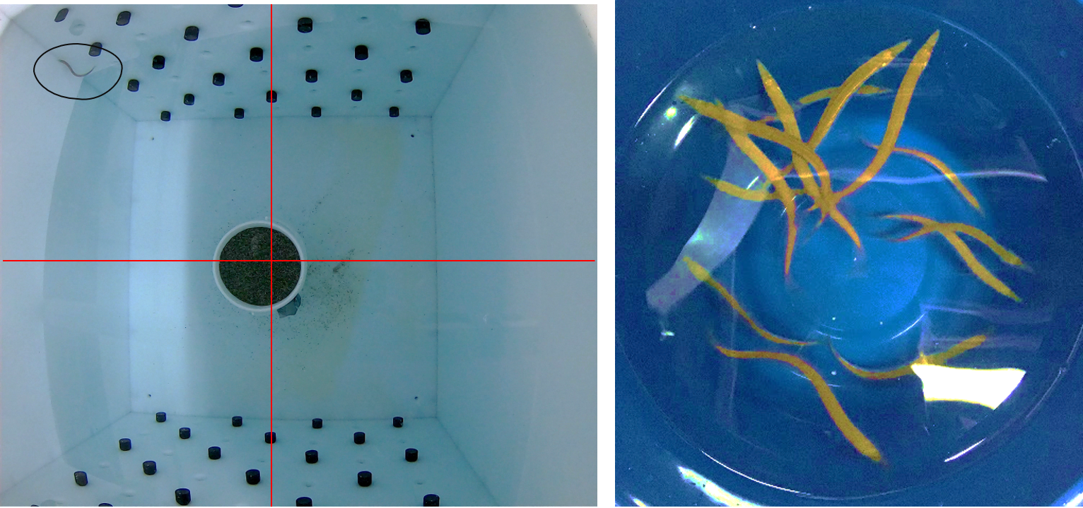
Figure 2. Left: Picture of the EMSS tank set up a bucket of sand in the center and a sand eel (black circle). The red axes delimit the quadrants which were used to describe the behavior of the fish. Right: Sand eels before testing.
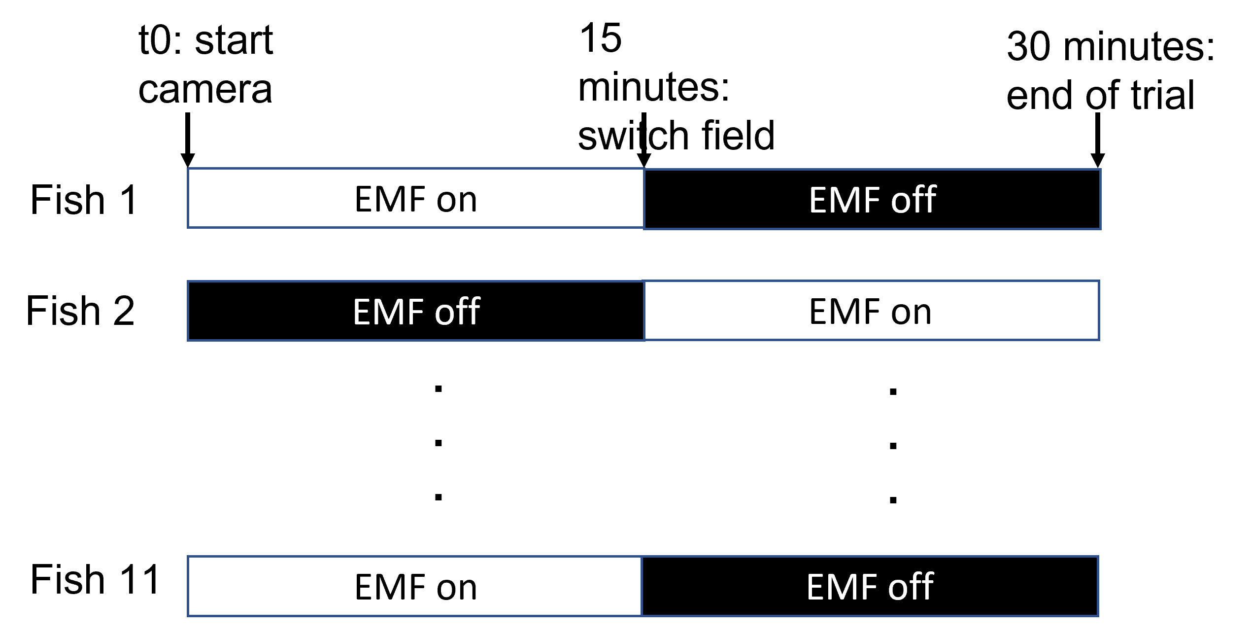
Testing took place over a 2-day period. The fish were collected from their housing tank, placed in a bucket, and moved to the testing location at the IMR research station. For each trial, one fish was placed in the EMSS tank and filmed for 30 minutes using a GoPro camera (Figure 2). A bucket of sand was placed in the bottom of the EMSS tank to provide the possibility of shelter for the fish. Each fish was subjected to two scenarios: EMF on and EMF off. We only tested level 3 EMF and exposures lasted for 15 minutes. The on/off sequences were alternated for each fish (Figure 3).
Figure 3. Schematic of the EMF testing protocol for sand eel.
2.2.2 - Video and statistical analyses
The tank was filmed from above and divided into quadrants. Time spent in the different quadrants of the tank were estimated from video observations. None of the fish sought refuge in the sand. Video time stamps were noted every time the fish changed quadrants. These were summed up for each trial and treatment to estimate the following variables:
Time spent in the different quadrants of the tank and in the center
Time spent searching the electrode area versus the blank walls
Time spent at the bottom, middle or surface of the water
Activity was defined as the number of times that the fish changed area (quadrant or center). The first 10 minutes were considered as an acclimation period and were not used in the analyses. The effect of the treatment on sand eel activity was tested using a Wilcoxon test. The other variables (times spent) were tested using a generalized linear mixed model using treatment as a fixed effect and individual fish as a random effect.
2.3 - Haddock experiment
2.3.1 - Description of protocol
Haddock ( Melanogramus aeglefinus ) is found in the North Atlantic Ocean and associated seas. Some of the largest stocks are found along the coast of Norway. Spawning takes place at depths of around 50 to 150 m. Adults were caught in Austevoll, offshore of IMR’s research station. Fertilized eggs were collected at the outlet of their holding tank and incubated. The juveniles used in the experiments hatched on March 19 and were 48 days old when tested.
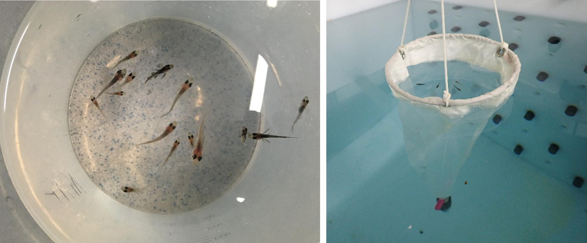
Figure 4. Left: Haddock juvenile before testing. Right: Haddock juveniles were placed in a plankton net in the EMSS tank for exposure to the different electromagnetic fields.
Tests occurred over a 2-day period. Groups of fish were exposed during the morning, then tested later in the day. Approximately 15-25 individuals were exposed at a time (Figure 4). For each trial, fish were carefully moved from the rearing tank into a plankton net which was hanging in the EMSS tank. The fish were exposed to different EMF levels (or not in the case of the control) for a duration of 15 minutes. These treatments corresponded to different configurations simulating different distances from the source (table 1): low field (level 1), strong field (level 2), or near field (level 3). After each exposure the larvae were transferred into plastic bottles which were placed in a cooler box, then transported by car to the MagLab. The sequences of the exposure treatments were different between both days (Table 2). The water temperature in the tank was 9.4 °C.
Day
1
Level 2
Control
Level 3
Level 1
2
Level 1
Level 3
Control
Level 2
Table 2. Sequence of exposure treatments
2.3.2 - Magnetic orientation facility (MagLab)
The MagLab was designed to test the ability of organisms to orient using the Earth’s magnetic field as a cue. The building is made of non-magnetic material and is located 300 m away from any road, building or power line which could cause some magnetic or other disturbance. A cube coil system is used to generate a magnetic field of the same intensity as the ambient field. It follows the design of Merritt et al. (1983), (see also Kirschvink, 1992) with a set of four double-wrapped coils. One coil is used to cancel the horizontal component of the ambient field and the remaining three coils are used to produce artificial magnetic fields matching the intensity and inclination of the ambient field and aligned in one of four directions with magnetic north at geographic north, east, south, or west. Total intensity inside the coil system was set to replicate as closely as possible total intensity of the ambient field and varied from 50.3 µT to 51 µT.
Date
trial
Treatment
Field
6-May-21
1
control
e
6-May-21
2
level1
e
6-May-21
3
level3
s
6-May-21
4
control
n
6-May-21
5
level2
w
6-May-21
6
level1
w
6-May-21
7
level3
n
6-May-21
8
control
s
6-May-21
9
level2
e
6-May-21
10
level1
s
6-May-21
11
level2
s
7-May-21
12
level3
e
7-May-21
13
control
n
7-May-21
14
level2
n
7-May-21
15
control
s
7-May-21
16
control
e
7-May-21
17
level3
w
7-May-21
18
level1
n
7-May-21
19
control
w
7-May-21
20
control/level 1
w
Table 3. Description and order of the tests carried out on haddock (Melanogramus aeglefinus ) juveniles (4 individuals per trial) in the MagLab.
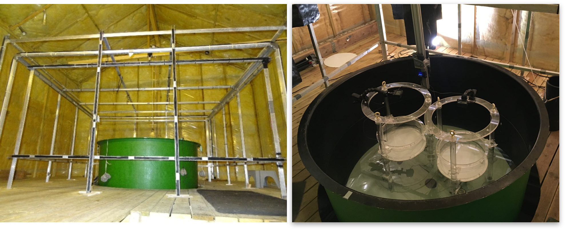
For each trial, four fish were carefully placed in observation chambers (2 fish per chamber) in the test tank inside the coil (Figure 5). The test tank is located inside the coil system and was filled with water pumped from the sea (300 m away from the building) prior to the tests. The water temperature in the tank varied between 10.4 and 10.8 °C during the trials. The circular observation chambers were 30 cm in diameter and lined with plankton mesh (Figure 5, right). GoPro cameras were attached on one side and recorded the movements of the animals during each trial. Each fish was tested only once, that is after each test they were replaced by a new set of four fish. An approximately equal number of trials were done in each of the four magnetic field alignments: north, south, east, west (table 3). We ran twenty trials (11 trials on 5/05/2021 and 9 trials on 6/05/2021. The sequence of treatment*magnetic field was randomized. Not all EMF exposed individuals (25 per day and per treatment) were tested. At the end of each day, left-over individuals were counted, and mortality was determined (table 4).
Figure 5. Magnetic orientation testing facility (MagLab). The cube coil (left) allows one to change the direction and intensity of the ambient magnetic field. Two testing arenas were used in the study (right). Each arena was lined with plankton mesh and was fitted with a camera. Four individual fish were tested per trial (two fish per area).
2.3.3 - Image and statistical analyses
We assumed that it took five minutes for the fish to acclimate to the arena and therefore removed the first five minutes of the videos before analyses, resulting in a 10-minute video. Videos were imported into Tracker 5.1.5. (Brown, 2020) as 600 images (1 frame per second). The software provides cartesian coordinates of the tracked ‘particle’ (here the fish), path lengths (in two dimensions), and instantaneous swimming velocities (over a 1 s interval). Polar coordinates were calculated from the x and y positions from which we derived a mean direction per fish. Mean vectors (r) per treatment were then calculated on these means (aggregated per fish) and Rayleigh tests were performed to evaluate whether mean directions were significant. “Magnetic bearings” were calculated by readjusting the directions according to the direction of the magnetic field (north, south, west, or east). For example, a fish having a topographical mean direction of 163°, and tested in the east field would have a magnetic mean direction of 163-90=73°.
We removed data when the fish was immobile (corresponding to instantaneous velocities (v) equal to 0) to analyze differences in instantaneous velocities (v). Even then, velocities (v) were skewed and therefore differences were tested using a generalized linear model (GLM) with a gamma distribution and a log link function. Differences in maximum distance travelled were analyzed using ANOVA. Fitness of the models was evaluated by examining the residuals vs. predicted values and QQ plots. All analyses were done in R. Tracking videos generates a very large amount of data (>10 000 observations). The results of studies based on large samples are often characterized by extreme statistical significance (Lantz, 2013). In such cases, the degree of significance can be determined from effect size which describes the observed relative divergence from the expectation specified in the null hypothesis (Lantz 2013). Here we calculated effect size as the difference between the two means (control and exposed) divided by the standard deviation of the data and used 0.20, 0.50, and 0.80 as benchmark values for small, medium and large effects respectively (Lantz 2013).
3 - Results
3.1 - Lesser sandeel
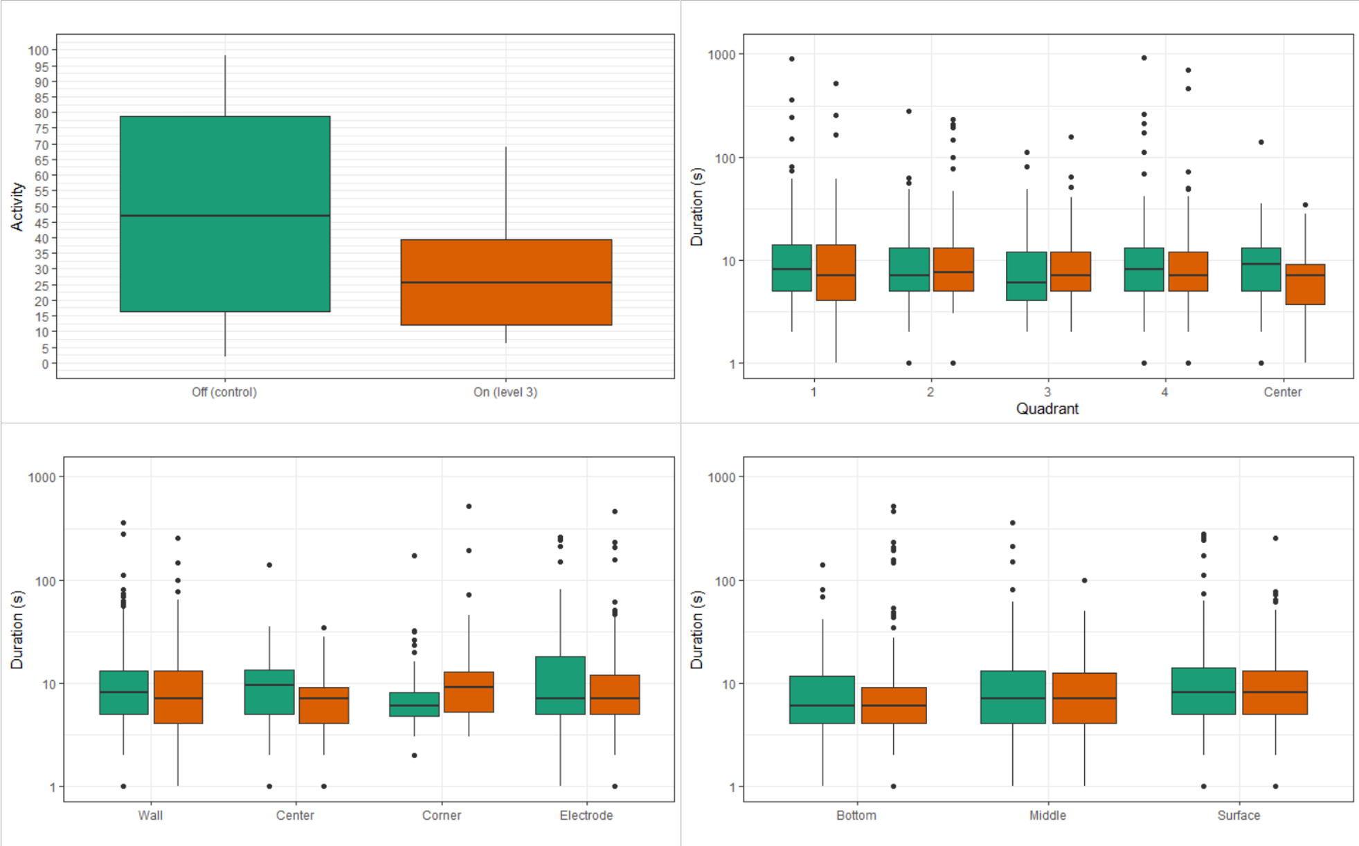
There was no mortality in the sand eels during or after the experiment. There was no significant difference between treatments (EMF on, EMF off), (Figure 6, p>0.1). Although, median activity appeared to be lower in the Off treatment (Figure 6), it was not statistically significant (Wilcoxon test, p=0.89).
Figure 6. Effect of Level 3 electromagnetic field (EMF) treatment on the behavior of sand eel (Ammodytes marinus) (n=11).
3.2 - Haddock
There was no significant relationship between EMF exposure and mortality (Table 4).
EMF exposure
Day 1
Day 2
Control (n=25)
2
3
Level 1 (n=25)
0
1
Level 2 (n=25)
0
0
Level 3 (n=25)
3
0
Table 4. Number of dead haddock ( Melanogramus aeglefinus ) juveniles at the end of each test day.
3.2.1 - Magnetic orientation
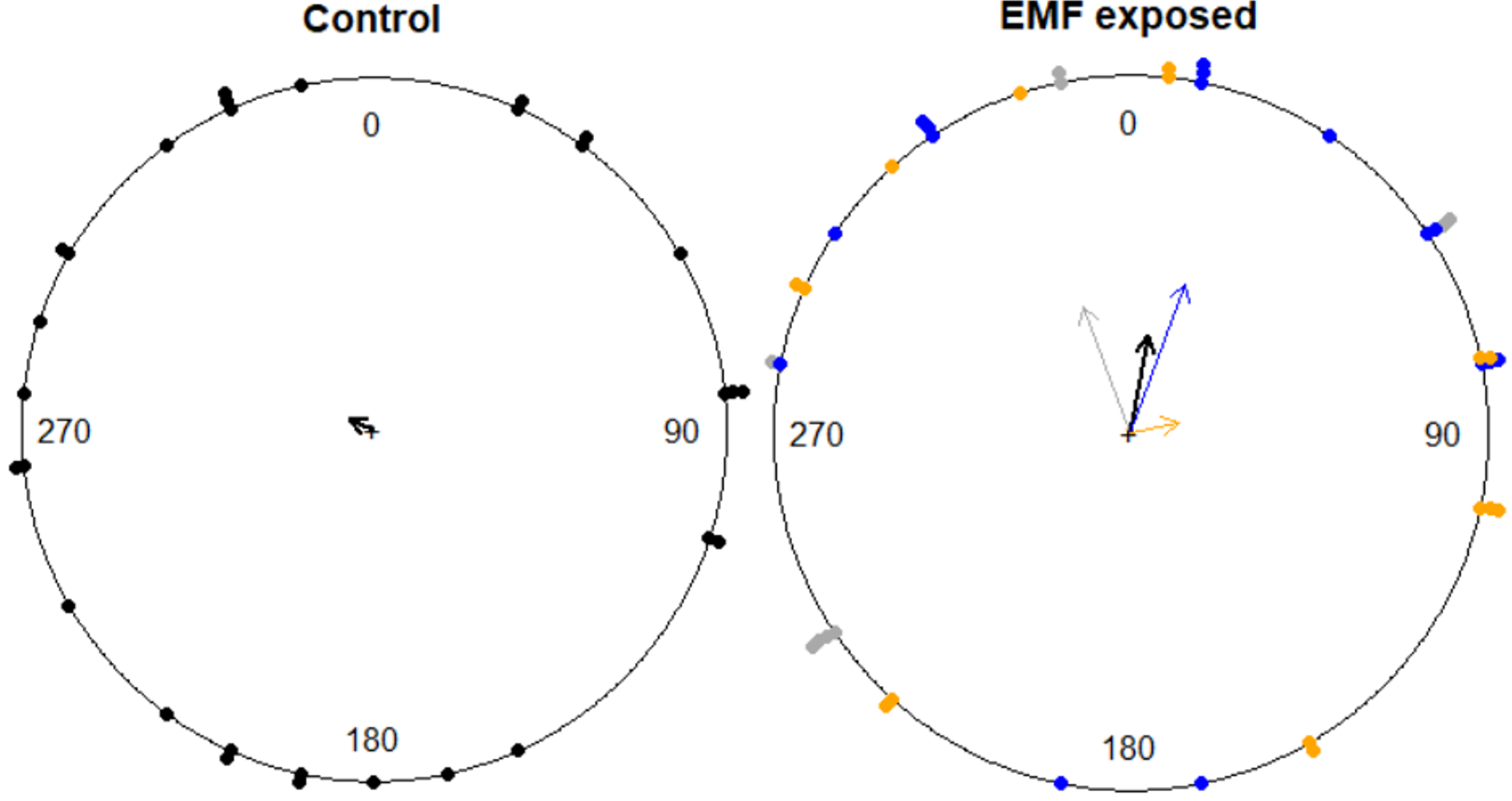
Results concerning magnetic orientation were unclear because the non-corrected (topographical) bearings showed a higher significance (r=0.32, n=80, p= 0.0004). In other words, fish seemed to orient, at least partly, according to a visual cue. However, orientation was also significant when corrected for the direction of magnetic north (r= 0.182, n=80, p=0.089) but only in EMF exposed fish and more specifically in fish exposed to levels 1 and 2 (Figure 7, Table 5).
Exposure treatment
Magnetic
Topographic
Control
r=0.079, n= 30, p=0.83
R= 0.35; n=30; p =0.026 **
Level 1
r=0.38, n= 16; p=0.10 *
R=0.43; n= 16; p=0.049 **
Level 2
r= 0.44, n=16; p=0.04 **
R=0.37; n= 16; p= 0.11
Level 3
r= 0.14; n= 15; p=0.76
R=0.25; n= 15; p=0.39
Table 5. Orientation of haddock ( Melanogramus aeglefinus ) larvae, Rayleigh test (r is the length of the mean vector, it measures angular dispersion and ranges from 0 to 1; p is the probability that the data are uniformly distributed)
Figure 7. Magnetic orientation of haddock (Melanogramus aeglefinus) juvenile exposed to EMF (n=30) or not (control, n=47). Arrows represent mean vectors (r). The black arrows represent the overall mean vector, while subgroups represent the EMF levels: level 1 (grey), level 2 (blue), level 3 (orange).
3.2.2 - Swimming velocities and distance travelled
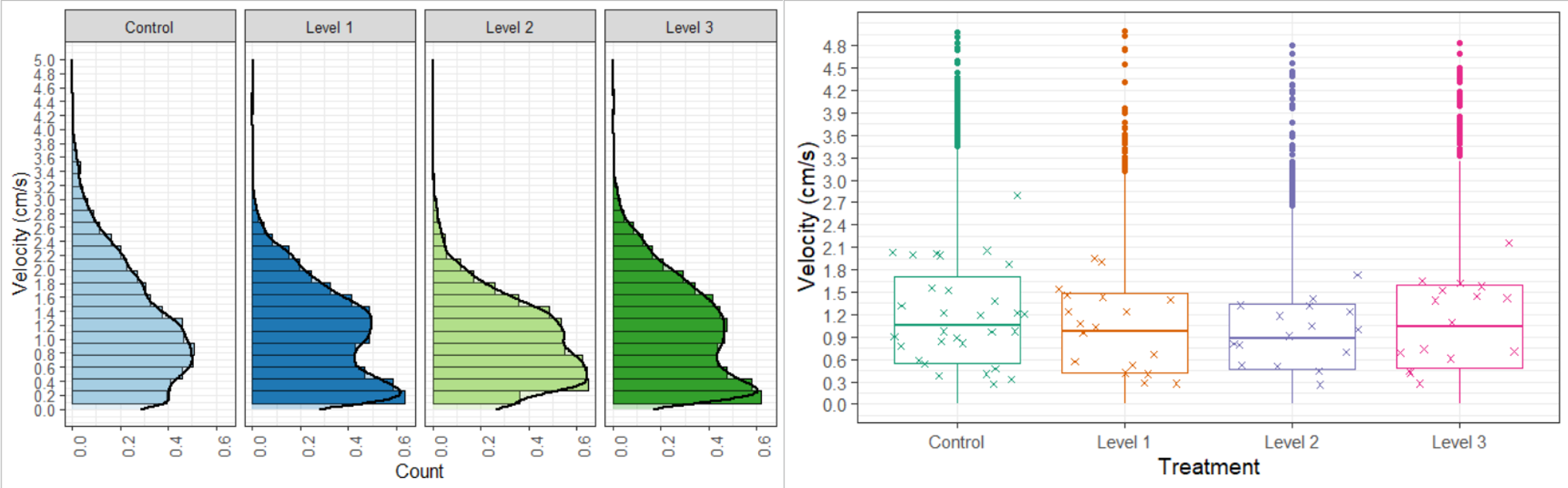
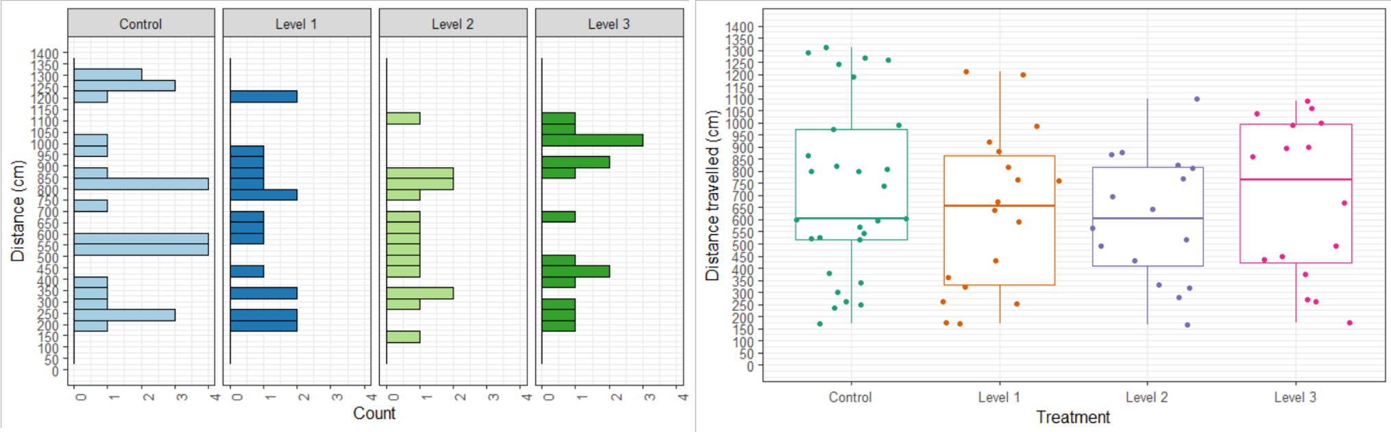
The exposure to EMF led to significant decreases in swimming velocity (p<0.0001), and with effect sizes between small and medium for level 1 (0.22) and level 2 (0.31) and almost no effect for level 3 (0.10). Mean instantaneous swimming velocities of haddock decreased from 1.18 pixel/s (control) to 0.86, 0.80 and 0.94 pixel/s after exposure to Level 1, 2 and 3 respectively (GLM estimates), representing speed reductions of 27%, 32% and 21% after exposure to each respective level. This decrease was due to a higher proportion of ‘slow individuals’ - displaying velocities < 0.8 pixel/s - in the treatment groups (Figure 8). This did not have a significant repercussion on the maximum distance travelled by a fish. The distance travelled during each trial was 644 cm (mean), and this did not significantly vary between EMF treatments (p=0.5) (Figure 9).
Mean velocities (pixel/s)
Confidence interval (2.5%-97.5%)
Effect size
Control
1.18
1.17-1.19
Level 1
0.86
0.85-0.87
0.22
Level 2
0.80
0.79-0.82
0.31
Level 3
0.94
0.92-0.95
0.10
Table 6. Estimated mean velocities of haddock ( Melanogramus aeglefinus ) after exposure to EMF (level 1: low, level 2: medium, level 3: high – see table 1 for corresponding simulated distances between the fish and the EMF source). The effect size is calculated according to Lantz 2013.
Figure 8. Instantaneous swimming velocities of haddock (Melanogramus aeglefinus) juvenile exposed to three levels of electromagnetic fields simulating different distances from the source. Control: ambient field, Level 1: 1000 m, Level 2: 100 m, Level 3: 30 m. Left: velocities are represented as histograms; Right: Boxplot calculated on all the individual velocities. Aggregated values (mean) per fish (n=80) are represented as crosses.Figure 9. Total distance travelled by haddock (Melanogramus aeglefinus) juvenile (n=80) exposed to three levels of electromagnetic fields simulating different distances from the source. Control: ambient field, Level 1: 1000 m, Level 2: 100 m, Level 3: 30 m. Left: Distances are represented as histograms; Right: Distances are represented as boxplots.
4 - Discussion and conclusion
We tested the effect of exposure to electromagnetic fields (EMF) used in surveys for oil and gas on two fish species (haddock and sandeel).
4.1 - Swimming velocity
We found that haddock juveniles had a significantly reduced swimming speed following exposure to the electromagnetic field generated in EM surveys. The effect was similar for field intensities equivalent to distances of 100 (Level 2) and 1000 m (Level 1) from the source with an average reduction in speed of 24%. The swimming velocity of adult European eel ( Anguilla anguilla ) also decreased when crossing the electromagnetic field of submarine power cable (Westerberg & Lagenfelt, 2008). The decrease was proportional to the electric current, although the relationship was weak. However, the decrease was more important in oil exposed fish, 30-40% (Cresci et al., 2020). Chemical changes may occur in the water in the EMSS tank when it is running due to electrolysis around the electrodes (Buchanan et al., 2011). For this reason, we changed the order of the exposure treatments and ensured that the control group (system off) was never exposed first. Therefore, the changes in swimming speed we observed cannot be due to changing water chemistry during the exposure period.
Static magnetic fields may affect the motor function of the cardiac muscle, by both increasing and decreasing the heart rate (Formicki et al., 2019), and by causing an increase in the frequency of movement of pectoral fins (Formicki, 1992; Winnicki & Formicki, 1990). Further research is needed to understand this change in behavior and especially on how long lasting this effect is. We can already conclude that the effect lasts for several hours after the exposure because, the exposure took place in the morning, between approximately 9 and 11 and recording of behavior occurred between 11:00 and 14:00. On day 1, Level 2 fish were exposed at 9:00 and tested up to 5 hours later. They had a mean velocity of 0.78 cm/s, which was still significantly lower than control fish (1.27 cm/s).
4.2 - Magnetic orientation
Haddock can orient according to the magnetic field (Cresci et al., 2019), and therefore we tested whether this ability was disrupted by exposing the fish to the EMF treatments. We found borderline significant magnetic orientation, but only in EMF exposed fish. Unfortunately, we did not visually shield the two test arenas from one another and this likely influenced the orientation of the fish, making it difficult to conclude with certainty. However, we did find significant magnetic orientation in Level 1 (p<0.1) and Level 2 (p<0.05) exposed fish. Moreover, the mean magnetic directions were similar in both arenas (figure 2, 339° and 20°) and similar to the data from Cresci et al. (2019): 319°. Interestingly, and as this was also the case for swimming velocity, there was no difference either between control or level 3. Therefore, a preliminary conclusion concerning magnetic compass orientation is that it appears that the fish rely more on magnetic cues after EMF exposure. Similarly, lobsters exposed to magnetic pulses significantly oriented while individuals in a control group (no magnetic pulse exposure) did not (Ernst & Lohmann, 2016). Such an effect is consistent with a type of magnetoreceptor which would be mediated by magnetic particles ( i.e . magnetite) (Kirschvink et al., 2001; Shaw et al., 2015) .
4.3 - Consequences of EMF exposure – upscaling to the population level
It is difficult to evaluate what consequences decreases in swimming velocities can have for juvenile haddock at the population level. Also, it is not known whether this is a physiological response, for example resulting from a decrease in heart rate or if it is a behavioral response to a change in the environment that the fish is sensing. In the latter case, exposed juveniles could very well increase their speed if required, i.e . in the presence of a predator or a prey. So, it is not possible to make unequivocal conclusions about detrimental effects with regards to their survival. However, swimming speed may affect dispersal of juveniles.
In contrast to lower intensity EMFs, Level 3 had a limited effect on haddock larvae. It is possible that these intensities correspond to an upper threshold level. This could constitute a mechanism to filter out erratic magnetic or electric noise out of the range of what is useful for these organisms that use the Earth’s magnetic field magnetic field to navigate (Buchanan et al 2011). Such a system would cause the organism to shut down magnetoreception during for example a solar storm, which would induce navigation errors. This may also be a reason why we did not find any effect of the Level 3 treatment on sand eel.
In conclusion, we found slight but significant effects on haddock larvae of the electromagnetic fields generated by subsea surveys. The EMSS tank is particularly well suited to test marine organisms, and follow-up experiments should be carried out to clarify effects on magnetic orientation following EMF exposure. In the present study, the swimming speed decrease was observed only a few hours after the exposure, but whether effects can last several days it should be investigated. Other pelagic fish species that could be exposed to such surveys should also be tested in a similar manner (for example, cod).
Buchanan, R., Fechhelm, R., Abgrall, P., & Lang, A. (2011). Environmental Impact Assessment of Electromagnetic Techniques Used for Oil & Gas Exploration & Production. LGL Rep. SA1084. by LGL Limited, St. John's, NL. In: Canada for International Association of Geophysical Contractors, Houston ….
Cresci, A., Paris, C. B., Browman, H. I., Skiftesvik, A. B., Shema, S., Bjelland, R., Durif, C. M. F., Foretich, M., Di Persia, C., Lucchese, V., Vikebo, F. B., & Sorhus, E. (2020). Effects of Exposure to Low Concentrations of Oil on the Expression of Cytochrome P4501a and Routine Swimming Speed of Atlantic Haddock (Melanogrammus aeglefinus) Larvae In Situ. Environmental Science & Technology, 54(21), 13879-13887. https://doi.org/10.1021/acs.est.0c04889
Cresci, A., Paris, C. B., Foretich, M. A., Durif, C. M., Shema, S. D., O'Brien, C. J. E., Vikebo, F. B., Skiftesvik, A. B., & Browman, H. I. (2019). Atlantic Haddock (Melanogrammus aeglefinus) Larvae Have a Magnetic Compass that Guides Their Orientation [Article]. Iscience, 19, 1173-+. https://doi.org/10.1016/j.jsci.2019.09.001
Ernst, D. A., & Lohmann, K. J. (2016). Effect of magnetic pulses on Caribbean spiny lobsters: implications for magnetoreception. Journal of Experimental Biology, 219(12), 1827-1832. https://doi.org/10.1242/jeb.136036
Formicki, K. (1992). Respiratory movements of trout [Salmo trutta L.] larvae during exposure to magnetic field. Acta Ichthyologica et Piscatoria, 22(2).
Formicki, K., Korzelecka-Orkisz, A., & Tański, A. (2021). The Effect of an Anthropogenic Magnetic Field on the Early Developmental Stages of Fishes—A Review. International Journal of Molecular Sciences, 22(3), 1210. https://doi.org/10.3390/ijms22031210
Formicki, K., Korzelecka‐Orkisz, A., & Tański, A. (2019). Magnetoreception in fish. Journal of Fish Biology. https://doi.org/10.1111/jfb.13998
Helwig, S. L., Wood, W., & Gloux, B. (2019). Vertical–vertical controlled‐source electromagnetic instrumentation and acquisition. Geophysical Prospecting, 67(6-Geophysical Instrumentation and Acquisition), 1582-1594.
Kirschvink, J. L. (1992). Uniform magnetic fields and double-wrapped coil systems: Improved techniques for the design of bioelectromagnetic experiments. Bioelectromagnetics, 13, 401-411.
Kirschvink, J. L., Walker, M. M., & Diebel, C. E. (2001). Magnetite-based magnetoreception. Current Opinion in Neurobiology, 11(4), 462-467.
Merritt, R., Purcell, C., & Stroink, G. (1983). Uniform magnetic field produced by three, four, and five square coils. Review of Scientific Instruments, 54(7), 879-882. http://link.aip.org/link/?RSI/54/879/1
Nyqvist, D., Durif, C., Johnsen, M. G., De Jong, K., Forland, T. N., & Sivle, L. D. (2020). Electric and magnetic senses in marine animals, and potential behavioral effects of electromagnetic surveys [Article]. Marine Environmental Research, 155, 11, Article 104888. https://doi.org/10.1016/j.marenvres.2020.104888
Robards, M. D., Willson, M., Armstrong, R. H., & Piatt, J. F. (1999). Sand lance: a review of biology and predator relations and annotated bibliography. Res. Pap. PNW-RP-521. Portland, OR: U.S. Department of Agriculture, Forest Service, Pacific Northwest Research Station. 327 p. (0882-5165). <Go to ISI>://WOS:000083507700002
Shaw, J., Boyd, A., House, M., Woodward, R., Mathes, F., Cowin, G., Saunders, M., & Baer, B. (2015). Magnetic particle-mediated magnetoreception. Journal of the Royal Society Interface, 12(110). https://doi.org/ARTN 20150499
10.1098/rsif.2015.0499
Westerberg, H., & Lagenfelt, I. (2008). Sub-sea power cables and the migration behaviour of the European eel [Proceedings Paper]. Fisheries Management and Ecology, 15(5-6), 369-375. https://doi.org/10.1111/j.1365-2400.2008.00630.x
Winnicki, A., & Formicki, K. (1990). Effect of constant magnetic field on myocardium activity in larvae of trout (Salmo trutta L.). Bulletin of the Polish Academy of Sciences. Biological Sciences, 38(1-12).
![Figure 1. Characteristics of the ElectroMagnetic Survey Simulator tank (EMSS tank). The magnetic field is induced by a set of wires mounted outside the holding tank (A). Ag/AgCl electrodes were mounted on plastic plates to generate the electric field (B, C). The signal generator controls the frequency of the magnetic and electric fields generated in the tank. The resistor box and power supply control the amplitude of the generated fields. The circular tank is 160 cm in diameter. The plastic frame holding the electrodes measures 86 x 85 x 110 [L x B x H cm].](/resources/images/nettrapporter/59883/file_html_3cdc6ff0c432b7f4.png)