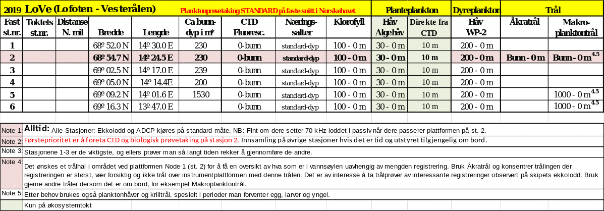
The overall aim of the survey was to collect data to support the CRIMAC center activities and the LoVe observatory. The survey was carried out on board GO Sars between the 26th of november and 3rd of December 2022 in the fjords and coastal areas off Troms including the overwintering areas of Norwegian spring spawning herring. The first part of the survey focused on further development of in trawl camera systems and data processing from such systems, testing and developing a trawl positioning system and fish detection and behavioural studies in front and inside the trawl using combined acoustic and optic methods. The second leg of the survey focused mainly on broadband acoustic data, including sizing of fish using broadbanded acoustics, noise estimation, calibration, time series consistency when changing to broad band acoustics, gas seep detection as well as performing the standard IMR LoVe transect. Eighteen scientists and technicians participated in the survey representing CRIMAC partner institutes Scantrol Deep Vision AS, Kongsberg Maritime AS, University of Bergen and Norsk Regnesentral in addition to IMR.
CRIMAC cruise report: Development of acoustic and optic methods for underwater target calssification
— G.O. Sars 22.11 - 03.12 2022
Report series:
Toktrapport 2023-3
ISSN: 1503-6294
Published: 09.03.2023
Cruise no.: 2022115
Project No.: 15662
On request by: Norges Forskningsråd
Reference: 309512
Research group(s):
Økosystemakustikk
,
Fangst
Program:
Marine prosesser og menneskelig påvirkning
Research group leader(s):
Rolf Korneliussen (Økosystemakustikk)
Approved by:
Research Director(s):
Geir Huse
Program leader(s):
Frode Vikebø
Norsk sammendrag
Summary
Hovedmålet med toktet var å samle data som støtter aktiviteter i CRIMAC senteret og LoVe observatoriet. Toktet ble gjennomført med forskningsfartøyet G.O. Sars 26.11 - 3.12.2022 i overvintringsområdene til norsk vårgytende sild i fjordene og kysten ved Troms. Første del av toktet fokuserte på videreutvikling og testing av Scantrol Deep Vision trålkamera inkluert dataprosessering, testing og utvikling av Kongsberg Maritimes trål posisjoneringssystem og målinger av fisk og atferd foran og i trålen ved bruk av kombinerte akustiske og optiske metoder. Andre del av toktet fokuserte hovedsakelig på bredbåndsakustiske data. Aktivitetene inkluderte størrelsesestimering av fisk ved bruk av bredbåndsakustikk, måling av støy og kalibrering av bredbåndsakustiske systemer, overgang fra smal til bredbåndsdata i rutine tokt, akustisk deteksjon av gasslekasje, samt gjennomføring av standard HI LoVe transekt. Med på toktet var 18 forskere og teknikere fra HI og CRIMAC partnerne Scantrol Deep Vision AS, Kongsberg Maritime AS, Universitetet i Bergen og Norsk Regnesentral.
1 - Introduction
The overarching objective of the survey is to collect data to support the CRIMAC activities and to collect data for the LoVe observatory. CRIMAC is a center of research-based innovation funded by the research council of Norway through their center for research-based innovation program (SFI). Sustainable, healthy food production and clean energy production for a growing population are important global goals, and CRIMAC will contribute to these by obtaining accurate underwater observations of gas, fish, nekton and other targets. The data will be used in conjunction with CRIMAC data from other surveys to build a reference data set for optical and acoustic target classification. The classification libraries will be used for developing methods and products toward the fishing industry and marine science. The survey was divided into two legs where leg one mainly focused on trawl instrumentation and data collection for behavioural studies on fish-trawl interactions. The main objectives of this part were to test in-trawl camera systems and data processing from such systems, test and develop trawl instrumentation and acoustic and optic monitoring of herring behaviour in relation to the trawl. The second leg of the survey focused mainly on broad band acoustic data, including sizing of fish using broad banded acoustics, noise estimation, calibration, time series consistency when changing to broad band acoustics, gas seep detection as well as performing the standard IMR LoVe transect.
2 - Survey overview
2.1 - Time period and area
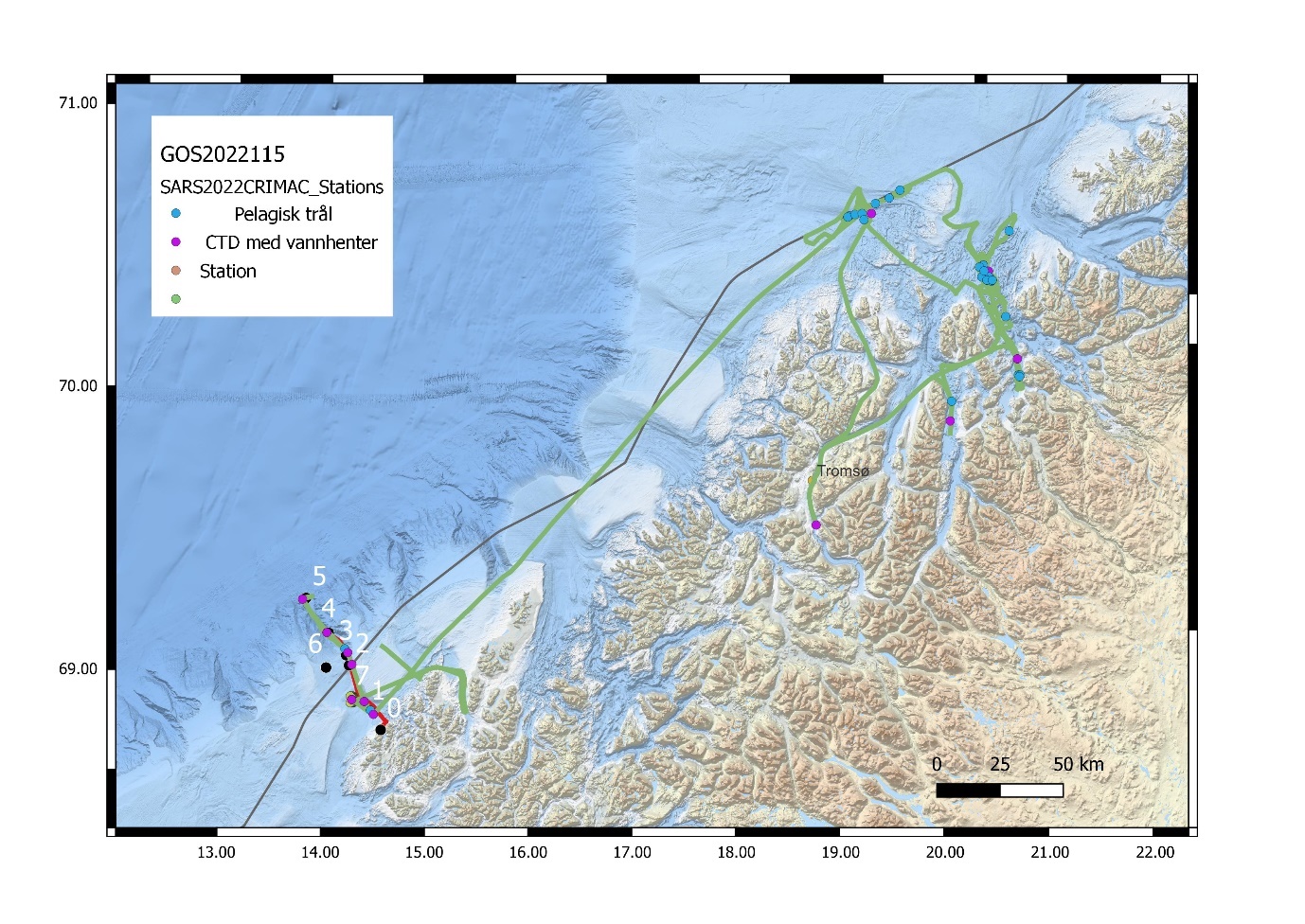
The first part of the cruise was conducted between November 22nd and November 26th with departing and ending in Tromsø. The second part was conducted between November 27th and December 3rd starting in Tromsø and ending in Myre. The survey area was inside the Lyngen, Reisa and Kvænangen fjords and along the coast off Tromsø (Figure 1). This includes the overwintering areas of the Norwegian spring spawning herring and a large coastal purse seine fleet were catching herring in the area during the cruise. In the second part of the cruise the LoVe transect was also covered. The major sampling stations, pelagic trawls and CTD as well as the survey track is shown in Figure 1.
2.2 - Data collection
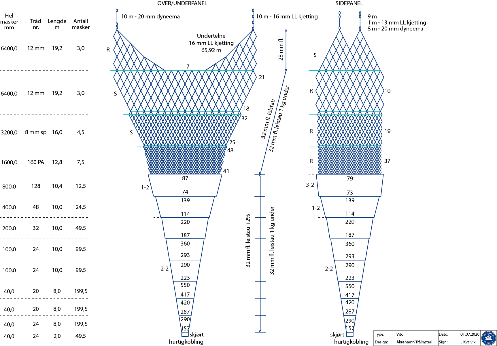
The IMR Vito pelagic sampling trawl with standard rigging and trawl monitoring instruments was used in all hauls (Figure 2). The trawl was spread with 8 m2 Thyborøn type 23 trawl doors with holders for both Simrad and Scanmar sensors. The door brackets were adjusted for pelagic trawling, with trawling warps attached to the top hole and bracket in the centre position. A Deep Vision codend (12 m long, 8 mm mesh liner) was used to collect physical samples. A split was made in the codend to limit catch sizes. The split was 1.3 m in length (2.0 - 3.3 m ahead of the codline) and sewn loosely closed with a thin twine dimensioned to break when the codend filled. To further limit catch size, constraining ropes were placed around the portion of the codend aft of the split to prevent it from filling completely. For the hauls without physical samples, the codend was simply left open.
2.3 - Vessel details
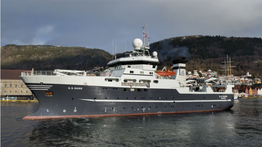
The cruise was conducted with RV G. O. Sars (Figure 3) operated by the Institute of Marine Research. The vessel is 77.5 m length overall, has a maximum speed of 17 knots and a crew of 15 in addition to space for 30 scientific crew members including instrument technicians. The vessel is equipped with Kongsberg Maritime EK80 scientific broadband echosounders (operating at 18, 38, 70, 120, 200, and 333 kHz centre frequency) and a range of other sensors (sonars, ADCPs). The vessel is equipped to deploy a wide range of additional equipment (e.g. probes, towed vehicles, pelagic and demersal trawls). More information about the vessel can be found online (https://www.hi.no/resources/brosjyre-g.o.sars.pdf).
2.4 - Cruise participants
| Scientific crew 1st part (22 – 26.11) | Scientific crew 2nd part (27.11 – 03.12) | ||
| Maria Tenningen | IMR | Nils Olav Handegard | IMR |
| Shale Rosen | IMR | Rolf Korneliussen | IMR |
| Jostein Saltskår | IMR | Geir Pedersen | IMR |
| Liz Kvalvik | IMR | Babak Khodabandeloo | IMR |
| Erik Schuster | IMR | Rokas Kubilius | IMR |
| Taraneh Westergerling | UiB | Leif Bildøy | KM |
| Eirik Svoren Osborg | Scantrol DV | Ingrid Utset | Norsk regnesentral |
| Jens Heinsdorf | KM | Ahmet Pala | UiB |
| Kameran Esmail | KM | ||
| Jon Even Corneliusssen | KM | ||
3 - Activities part I
In the first part of the cruise herring were detected inside the Reisafjord, outer edges of Kvænagen fjord and offshore at the 12 nm border (Figure 4). Herring were mainly observed in large layers that varied in density and depth. In general, the aggregations were closer to surface (25 – 100 m) and less dense in the evening and night. In the early morning herring density in the aggregations increased and the fish moved deeper (150 – 200 m). Four CTD casts were made in the main areas of trawling. We had in total 20 trawl hauls, five hauls with closed codend to obtain a physical sample of the catch (Table 2). In all trawl hauls the scientific Deep vision Camera system was used for monitoring catch composition. The FOCUS 2 underwater towed vehicle (MacArtney AS) was deployed in two of the hauls to make detailed observations of trawl and trawl intsrumentation (e.g. Scantrol DV camera system) performance using the camera and scanning sonar mounted on the vehicle.
| Haul | Date | Lat (N) | Lon (E ) | Time start | Time end | Trawl depth | Instrumentation | Trawl sample (herring) | Comment | |||||
| WBAT | Dark Vision | Fisheries DV | Research DV | Focus | L (mm) | W (kg) | ||||||||
| 489 | 22.11 | 69°54’ | 20°26’ | 21:46 | 23:47 | 165 | X | X | X | X | ||||
| 490 | 23.11 | 70°10’ | 21°01’ | 05:27 | 06:10 | 120 | X | X | X | X | 305 | 0.263 | Red light Dark vision | |
| 491 | 23.11 | 70°22’ | 20°54 | 08:58 | 09:42 | 160 | X | X | X | |||||
| 492 | 23.11 | 70°19’ | 20°55‘ | 14:26 | 15:13 | NA | X | X | X | |||||
| 493 | 23.11 | 70°28’ | 21°12’ | 18:41 | 19:42 | 250 | X | X | Fisheris DV malfunction | |||||
| 494 | 24.11 | 69°58’ | 21°09’ | 03:00 | 04:07 | NA | X | X | X | |||||
| 495 | 24.11 | 69°58’ | 21°10’ | 06:31 | 06:37 | 65 | X | 302 | 0.269 | (large herring catch) | ||||
| 496 | 24.11 | 70°18’ | 20°58’ | 12:17 | 15:00 | NA | X | X | X | X | X | Very good data from the whole trawl | ||
| 497 | 24.11 | 70°19’ | 20°57’ | 19:06 | 19:39 | 100 | X | X | X | 270 | 0.192 | Wbat cw | ||
| 498 | 24.11 | 70°21’ | 20°51’ | 21:47 | 22:17 | 80 | X | X | X | |||||
| 499 | 24.11 | 70°19’ | 20°52’ | 23:54 | 00:39 | 150 | X | X | X | First 30 min at 70 m | ||||
| 500 | 25.11 | 70°18' | 20°55' | 06:30 | 07:00 | 90 | X | X | X | X | ||||
| 501 | 25.11 | 70°20' | 20°54' | 08:58 | 09:29 | 190 | X | X | X | X | ||||
| 502 | 25.11 | 70°18' | 20°58' | 11:12 | 13:39 | 170 | X | X | X | X | Monitoring fish between doors and trawl wires | |||
| 503 | 25.11 | 70°39' | 20°09' | 18:47 | 19:17 | 84 | X | X | X | X | ||||
| 504 | 25.11 | 70°37' | 19°58' | 20:47 | 21:17 | 100 | X | X | 200 | 0.083 | ||||
| 505 | 25.11 | 70°34' | 19°31' | 22:41 | 22:54 | 72 | X | X | X | X | 259 | 0.142 | ||
| 506 | 26.11 | 70°34' | 19°30' | 00:10 | 00:39 | NA | X | X | X | X | ||||
| 507 | 26.11 | 70°34' | 19°35' | 05:58 | 06:47 | 110 | X | X | X | X | First 25 min at 53 m | |||
| 508 | 26.11 | 70°34' | 19°42' | 08:56 | 09:13 | 300 | X | X | X | |||||
3.1 - Detecting and measuring individual fish inside the trawl with combined camera and acoustic methods
Maria Tenningen (IMR)
Objective
The aim of this activity was to first test the feasibility of collecting data using a combination of scientific echosounder and a camera system mounted in the trawl. If this proved successful, the aim was to collect data for acoustic measurements of individual fish length and validate the acoustic data with in-trawl camera images. In pelagic fisheries target schools are usually monitored with sideways looking sonar and being able to estimate fish length before catch would be very useful when making decision before catch.
Method
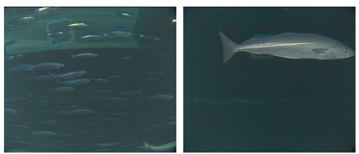
An autonomous wideband transceiver, Simrad WBAT (KM) with a 200 kHz wideband transducer (160 – 270 kHz) was attached in the trawl (Figure 5). The wbat was placed inside a protective housing and attached in the vertical center of the starboard side panel of the Vito sampling trawl at the junction between 400 and 800 mm meshes. The trawl opening in this position was measured to be 19.5 m horizontal and 8 m vertical (FOCUS sonar measurement). On the opposite side of the trawl the "Dark Vision" (IMR) camera system was attached (Figure 5). This is a camera system based on exsiting modules, built to be light senistive and programmable to collect video or images as needed (pers. comm. Sigurd Hanaas, IMR). In the first hauls red light was used not to disturb the fish, but due to very poor visibility we removed the red light filter and used white light for better range visibility (Table 2). The times of the wbat and camera system were synchronized. Data were collected in 17 hauls with different densities of fish, mainly herring but also saithe, mesopelagic, shrimp etc. The Deep vision camera collected image data further back in the trawl. Wbat settings are presented in table 3.
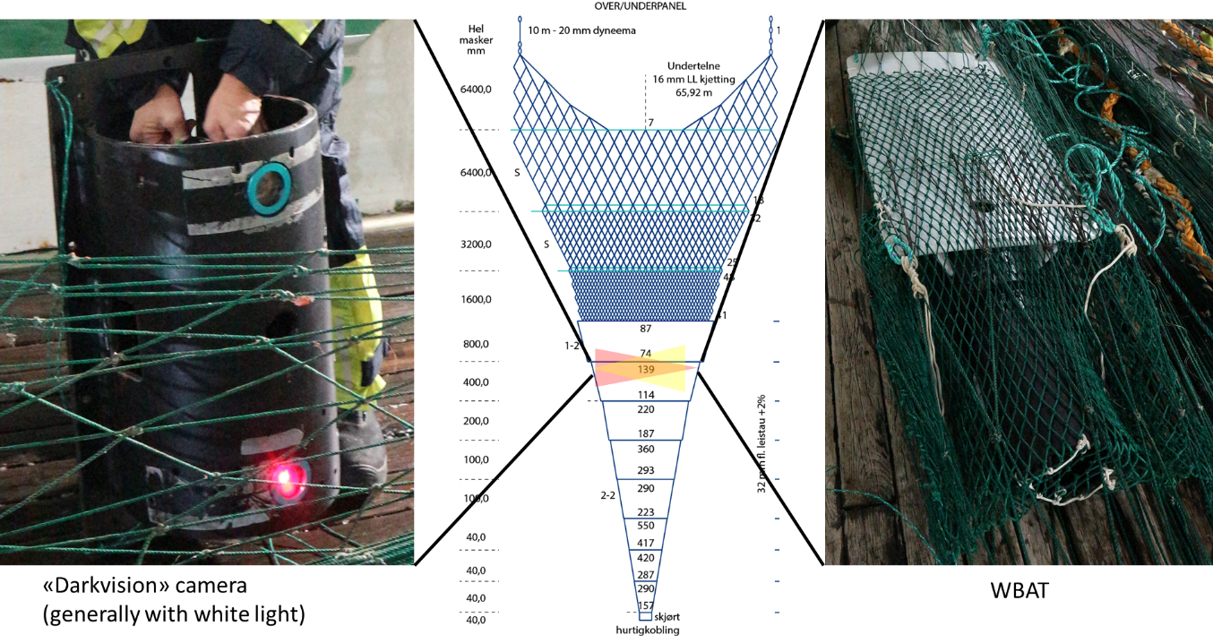
| Pulse form | Bandwidth, kHz | Taper | Pulse duration, ms | Power, W | Ping rate | Range | Hauls |
| FM-up | 170 – 260 | Fast | 2.048 | 105 | 0.5 | 25 | All except 493, 495, 497, 504 |
| CW | 200 | Fast | 0.256 | 75 | 25 | 497 |
Preliminary results
Based on a preliminary data scrutiny it is clear that individual targets can be detected in the acoustic data and fish are also clearly observed in the camera images (Figure 6). However, fish densities varied greatly between hauls and in the most dense concentrations it may be difficult to detect indivdiual fish. The dark vision camera did also not cover the whole range across the trawl and with the red light visibility was very poor. The white light provided better visibility, but may have affected the fish behaviour by attracting the fish close to the camera. A better solution to using the dark vision camera may be to use the data from the scientific deep vision further back in the trawl. The next step is to calibrate the wbat, then investigate the quality of the acoustic data and number of targets that can be detected. We will then decide how to continue with this work.
3.2 - Processing data from Deep Vision camera system
Taraneh Westergerling (UiB)
Objective
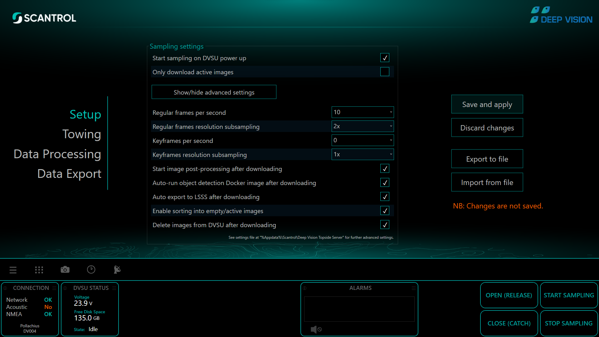
The Deep Vision system is planned to be used in some of IMRs stock assessment surveys. During these cruises, the instrument personnel and crew carry full responsibility for the data collection. In the past years, programmers from both Scantrol Deep Vision and IMR have worked on automating and speeding up the download process with the goal of utilizing the images during acoustic scrutinization. To ensure the applicability of the pipeline it is essential for it to run smoothly and not limit further data collection.
Method
A total of 20 Deep Vision sessions were recorded. From these 15 were collected using the standard settings (filtered, zipped, 10 fps, half resolution, no keyframes), 2 were recorded with full resolution, and 3 were unzipped and with full resolution (Table 4).
Attempts to run the full pipeline (download, post-processing, docker, export to LSSS, delete after download) failed. There were two main reasons for this: The first reason was that the docker, that contains the species identifiaction algorithm, was estimated to take 8h for each session. This was irrespective of file size. Consequently, we needed to remove that step from the pipeline. The second reason was that the “delete after download” box was not checked, this led to the deleting of unprocessed sessions on the topside PC. All sessions recorded from the first leg of the survey did therefore not run through the object detection network built by Allken et al. (2019).
The download time and post-processing time were recorded for all 17 zipped sessions, by observing the Topside HMI interface or by tracking the time stamp when the folders were created.
| Settings | Pipeline steps | ||||||||||||
|---|---|---|---|---|---|---|---|---|---|---|---|---|---|
| Station | Session | File size (GB) | Number of files | Filter | Zip | Frames per second (fps) | resolution | Keyframes | Download | Post-processing | Docker | Export to LSSS | Delete after download |
| 489 | 20221122T1928Z | NA | NA | no | unzipped | 10 | full | 0 | NA | NA | NA | NA | NA |
| 490 | 20221123T0409Z | NA | NA | no | unzipped | 10 | full | 0 | NA | NA | NA | NA | NA |
| 491 | 20221123T0813Z | NA | NA | no | unzipped | 10 | full | 0 | NA | NA | NA | NA | NA |
| 492 | 20221123T1347Z | 53.7 | 563 | yes | zipped | 10 | full | 0 | yes | yes | no | yes | yes |
| 493 | 20221123T1810Z | 51.6 | 562 | yes | zipped | 10 | full | 0 | yes | yes | no | yes | yes |
| 494 | 20221124T0225Z | 16 | 618 | yes | zipped | 10 | half | 0 | yes | yes | no | yes | yes |
| 495 | 20221124T0606Z | 12.1 | 355 | yes | zipped | 10 | half | 0 | yes | yes | partially | yes | yes |
| 496 | 20221124T1137Z | 29.1 | 1135 | yes | zipped | 10 | half | 0 | yes | yes | partially | yes | yes |
| 497 | 20221124T1825Z | 12.9 | 507 | yes | zipped | 10 | half | 0 | yes | yes | partially | yes | yes |
| 498 | 20221124T2048Z | 14.8 | 547 | yes | zipped | 10 | half | 0 | yes | yes | no | yes | yes |
| 499 | 20221124T2320Z | 15.5 | 507 | yes | zipped | 10 | half | 0 | yes | yes | no | yes | yes |
| 500 | 20221125T0545Z | 15.4 | 563 | yes | zipped | 10 | half | 0 | yes | yes | no | yes | yes |
| 501 | 20221125T0817Z | 13.3 | 515 | yes | zipped | 10 | half | 0 | yes | yes | no | yes | yes |
| 502 | 20221125T1033Z | 28 | 1030 | yes | zipped | 10 | half | 0 | yes | yes | no | yes | yes |
| 503 | 20221125T1803Z | 11.9 | 479 | yes | zipped | 10 | half | 0 | yes | yes | no | yes | yes |
| 504 | 20221125T2025Z | 8.88 | 355 | yes | zipped | 10 | half | 0 | yes | yes | no | yes | yes |
| 505 | 20221125T2211Z | 8.17 | 327 | yes | zipped | 10 | half | 0 | yes | yes | partially | yes | yes |
| 506 | 20221125T2340Z | 14.9 | 814 | yes | zipped | 10 | half | 0 | yes | yes | no | yes | yes |
| 507 | 20221126T0522Z | 12.9 | 515 | yes | zipped | 10 | half | 0 | yes | yes | no | yes | yes |
| 508 | 20221126T0816Z | 12.1 | 495 | yes | zipped | 10 | half | 0 | yes | yes | no | yes | yes |
Preliminary results
Since the Deep Vision system is used on both G. O. Sars and other vessels which do not host a pipeline there is a risk that camera settings are not kept constant. This was the case with the first 3 sessions that were collected in an unzipped format.
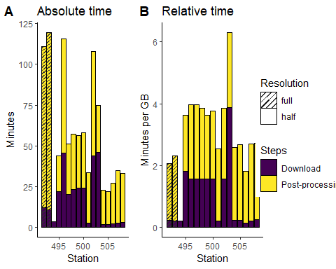
It is important to note that for now standard settings must be kept in order to run the pipeline smoothly Figure 7.
Download speed varied between stations and did not depend on file size Figure 8(A). It is not yet clear what lead to the extremely quick downloads of less than 4 minutes Figure 8(B). Post-processing on the other hand showed a clear correlation with file size Figure 8(B).
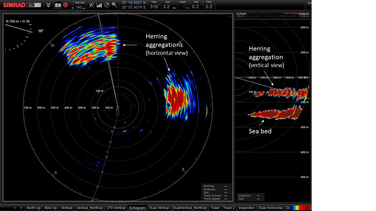
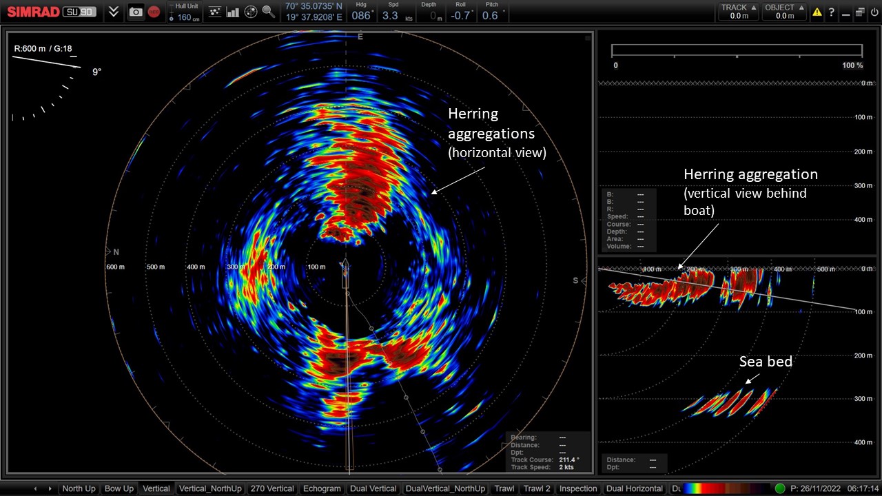
3.3 - Monitor herring school reactions to the vessel and trawl with multibeam fisheries sonar
Maria Tenningen (IMR)
Objective
The objective of this activity was to collect sonar data for describing how herring schools react to the vessel and the trawl. This activity is related to trawl positioning systems (section 3.6.) and an MSc project that aims to investigate how accurately acoustic registrations in scientific surveys are sampled by trawl with the following sub-objectives:
1. Describe school behaviour (relative density, school speed, depth and swimming direction) ahead of boat and between boat and trawl opening
2. Can we identify environmental or biological factors that affect behaviour (e.g. school size, individual size, school depth, weather, ambient light)?
3. Can better control of trawl position relative to fish school improve catch success?
Method
Data were collected with the Simrad SU90 fisheries sonar. A search range of 800 -1000 m was used and once an aggregation of herring was detected on the sonar the vertical beams were directed toward the fish aggregation to obtain depth distribution. The aggregation was then followed as G.O. Sars passed over the fish and in most cases trawled on the fish. The plan is to analyse the data to investigate whether the vertical distribution, acoustic backscatter strength (indicating a change in fish density or behaviour) or swimming direction changes first as the vessel passes over the school and then as the trawl targets the aggregation. The sonar based behavioural data can then be combined with biological information on length distribution and school size and information about trawl position.
Preliminary results
Several large herring schools or aggregations were monitored with the sonar (Figure 9). Some of the schools were also passed over by the boat and trawled on. The schools were monitored with the horizontal and vertical beams (Figures 9 and 10). The data can be used to investigate changes in depth and in acoustic backscatter strength (indication of spatial density and / or behaviour) as the vessel passes over the school and when the trawl approaches. However, it was challenging to follow the large layers and this activity would work better on smaller distinct schools.
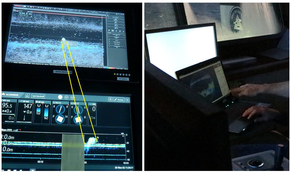
3.4 - Fish behaviour from trawl opening to codend
Shale Rosen (IMR)
Objective
The aim of this activity was to establish the passage rates of fish in front of and through the trawl. This is important when considering how the trawl’s path and images are integrated with echograms. Presently, the trawl path is positioned based upon average distance behind the vessel and assumes that fish are passive (neither swim with nor against the direction of trawling direction). This is in some ways an extension of the activity to monitor school behaviour between the boat and trawl opening. It was similarly challenged by lack of suitable fish aggregations (small, distinct schools).
Method and preliminary results
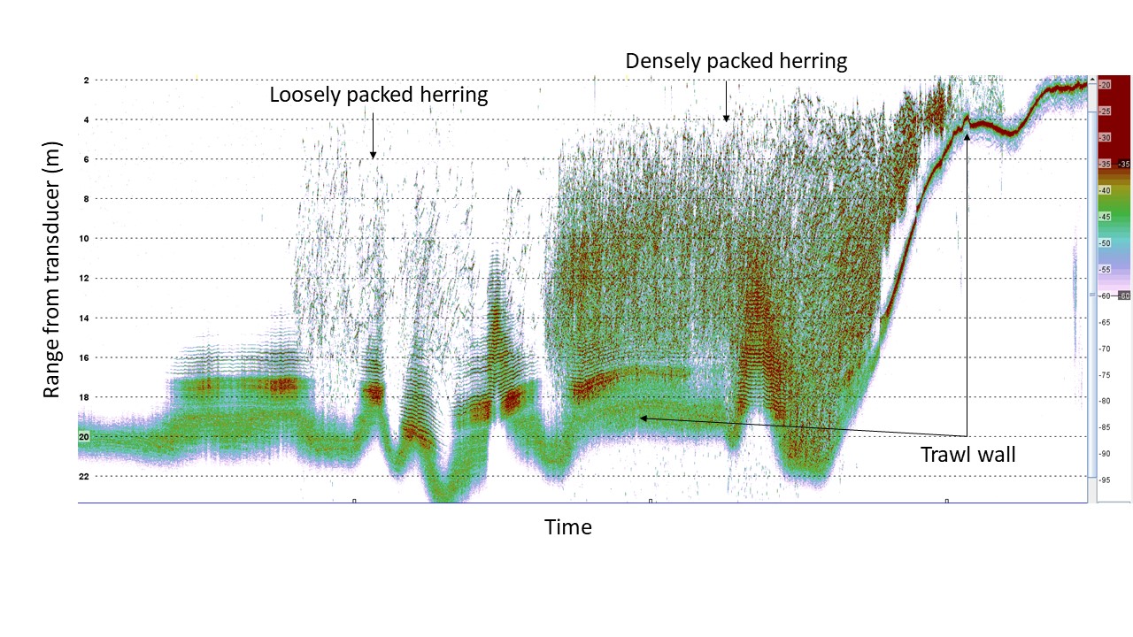
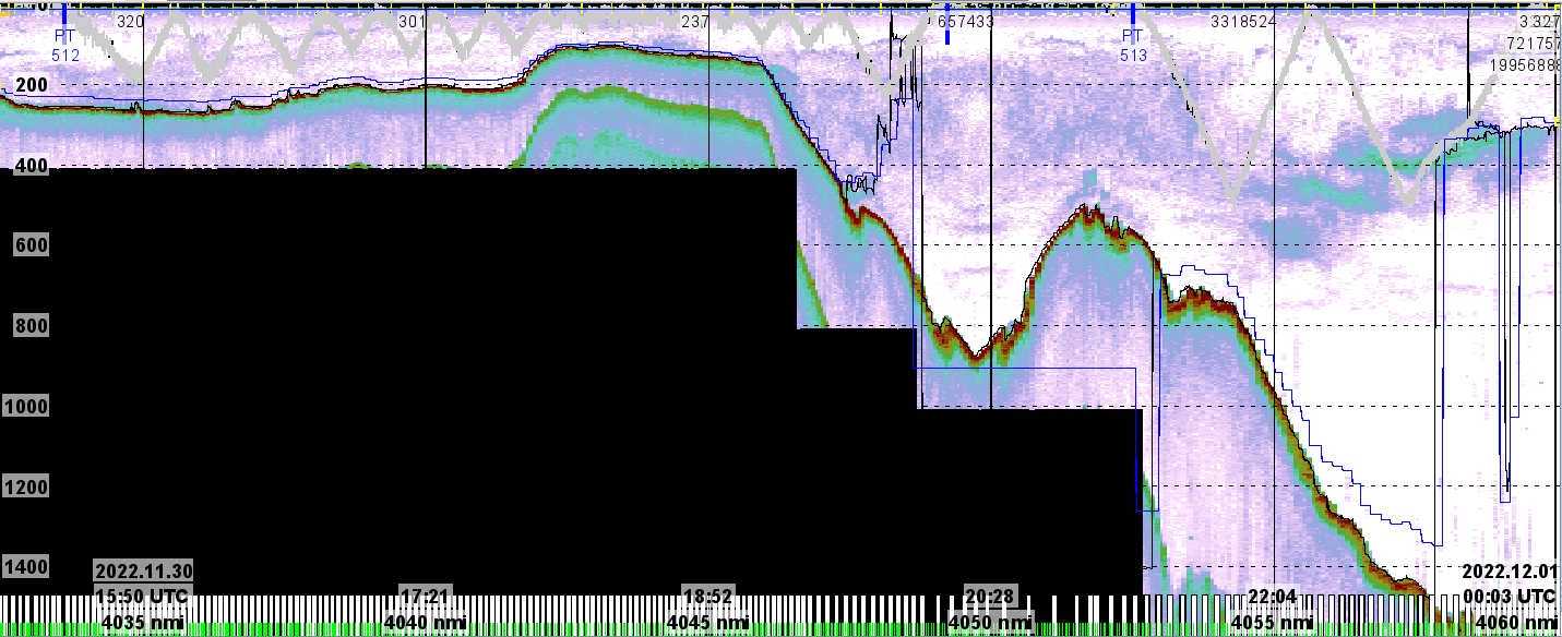
An experiment was carried out 25.11 (station PT where the FOCUS2 towed vehicle was positioned between the trawl doors and its scanning sonar was used to detect passing schools. The leading and trailing edges of the schools were detected again at the trawl opening using a Scanmar trawleye and should be visible again in the WBAT and both Deep Vision systems (Figure 11). Lights on the FOCUS were turned off and the Darkvision camera system was not used in conjunction with the WBAT in order to minimize the effect of artificial light (lights necessary for Deep Vision systems).
The echogram from the Scanmar trawleye is not recorded and the Simrad trawl eye could not be used due to interference with the WBAT (both operate at 200 kHz and interference was confirmed during earlier hauls). Therefore, the timing of entrances on the Scanmar trawleye were noted manually and documented by photographing the display.
It is unlikely that there is sufficient data for a full analysis to support this investigation at all of the locations. However, there is likely sufficient data to carry out an analysis of passage rates inside the trawl from the position of the WBAT (58 m into trawl) to the research Deep Vision (125 m into the trawl). This encompasses the aft 53 % of the trawl from headrope to beginning of the codend. Since analysis of passage times in WBAT and Deep Vision systems were not carried out, no preliminary results are available beyond those presented in Table 5.
| School number | SU90 sonar | EK80 | FOCUS at trawl doors | Trawleye | WBAT | Fisheries Deep Vision | Research Deep Vision |
| In front of vessel | Beneath vessel | Trawl doors (90 m ahead of trawl entrance) | Trawl entrance | 58 m into trawl | 118 m into trawl | 125 m into trawl | |
| 1 | 11:09:26-11:16:17 | Data not analyzed (not available in real-time) | |||||
| 2 | 11:24:15 (300 m range) | 11:27:20 | 11:31:50-11:42:50 | ||||
| 3 | 12:13:05 (400 m range, 130 m depth) | 12:20:37 | 12:24:05 | 12:24:36 | |||
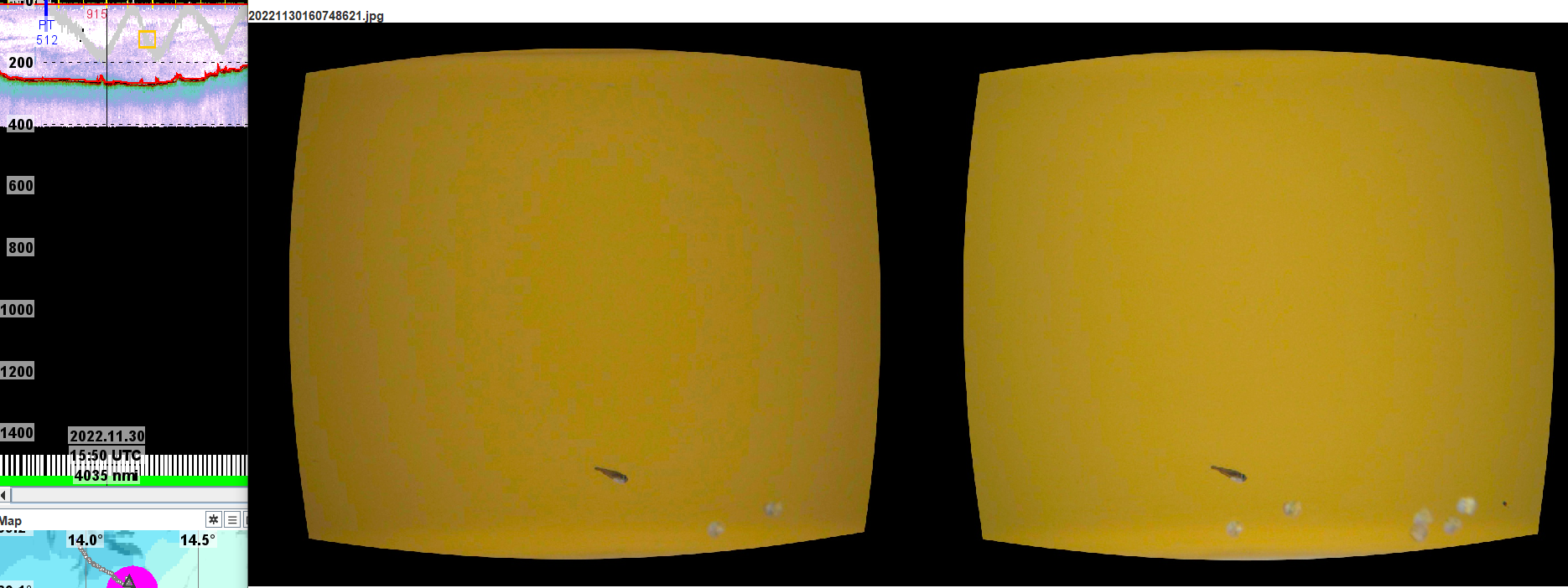
3.5 - Test and develop the commercial fisheries version of the Deep Vision camera system
Eirik Svoren Osborg (Scantrol DV)
Objective
A prototype for the Deep Vision Fisheries version was made ready for the CRIMAC survey in the fjords around Tromsø. The aim during the survey was to collect in-trawl images with a prototype Deep Vision system for knowledge and testing to the coming Deep Vision system for commercial fisheries. In addition to image collecting, Scantrol Deep Vision AS were also gathering information about how such a system can be designed for easy handling when shooting and heaving and positioning in the trawl.
Method
The Deep Vision Fisheries prototype camera system was built into a jig with lights and batteries and mounted in the middle of the last section of the VITO pelagic trawl (Figure 12). Different camera settings, light angles and intensities were tested. On some trawl stations, a fine mesh white netting was also installed on the panel opposite of the camera system to compare light and image differences.
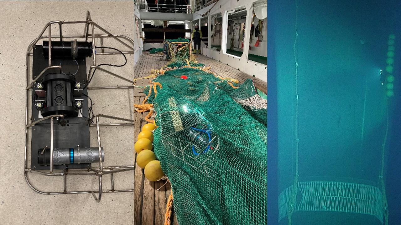
Preliminary results
The prototype was used to collect images on ten trawl stations. Three of these were with a white background, and the rest without any addition to the trawl. The images have been collected and will be further compared. However, a brief look through the images tells us that we have images of Atlantic Herring, Saithe and a few Cod that can be compared to images from the scientific Deep Vision model (Figure 13).
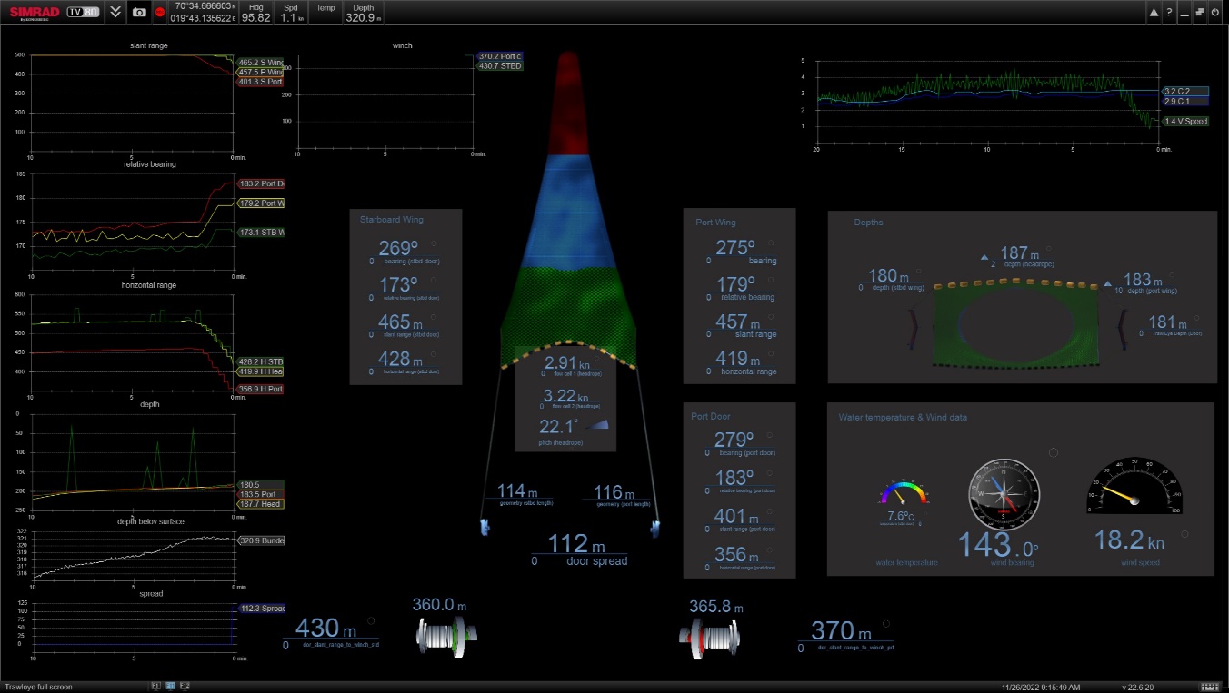
3.6 - Test and develop trawl door positioning system
Jens Heinsdorf (KM)
Objective
Knowing the location of the gear can be beneficial for fishing in several ways. Knowing the exact location of the trawl can help fishers target their fishing efforts more effectively. This can help them catch the right species of fish, at the right size and in the right quantities. Furthermore, knowing the location of the trawl gear in relation to the vessel can be an aid to safe navigation. The trawl might not always be in the same direction as the direction in which the warps leave the vessel. In e.g., areas where fishing vessels are crossing each other’s tracks or passing in proximity, knowing the actual location can help reducing the risk of collision and increase safety. Finally, it can help fishers comply with fishing regulations. Many areas have restrictions on where and when fishing can take place, and these regulations are in place to protect fish populations and the marine environment. By knowing the exact location of their trawl, fishers can ensure that they are fishing in compliance with these regulations.
Simrad PxPos sensors makes it possible to geo locate gear below the surface, using true latitude and longitude coordinates, as well as relative beading from the vessel. The acoustic response from the Simrad PxPos sensors is used to determine relative bearing to the sensors and the slant range (distance between transducer on the vessel and sensor). Together with measurements of depth, the vessels actual heading and vessel GPS position, the actual WGS84 GPS coordinates are calculated for each Simrad PxPos sensor. Installing Simrad PxPos sensor on the trawl gear hence makes it possible to know the exact location of both trawl doors and trawl net.
The aim of this activity was to verify that the system functions as intended and collect data for post-processing.
Method
Three Simrad PxPos sensors, two PX MultiSensors, one PX Flow Sensor, one PX TrawlEye and one PX miniCatch sensor were mounted on the IMR Vito pelagic sampling trawl in different configurations throughout the trip. The trawl doors were fitted with door brackets allowing for installation of two Simrad sensors in each door. In order to test different combination of sensors measurements, the Simrad PxPos and Simrad PX Sensors were configured so trawl geometry (distance between headline and trawl doors) was measured between Simrad PxPos and either PX Flow, PX MultiSensor or PX TrawlEye. Trawl door spread (distance between doors) was measured between Simrad PxPos and Simrad PxPos Remote sensor. Simrad sensors were in addition used to measure simultaneous depth of both trawl doors and the headline. Simrad PX miniCatch and Simrad PxPos sensors were also installed on the cod-end section during some of the hauls, while PX Flow in several hauls were installed on the headline and PX TrawlEye either in headline or in one of the trawl doors.
Simrad TP90 Trawl Positioning transceiver was provisionally installed on GO Sars using the already installed trawl positioning transducer. The SR70 Receiver Unit for Simrad PX, was installed using the onboard Scanmar hydrophone. Both The TP90 and SR70 were then connected to TV80 Trawl Software. Between the hauls, TV80 was used to change configuration of both Simrad PX and Simrad PxPos sensors. TV80 was as well configured to receive data from the onboard Gyro, onboard GPS, data from Simrad Echo Sounder and winch information from the Scantrol system.
| Haul | Date | Lat (N) | Lon (E ) | Time start | Time end | Simrad Sensors used |
| 489 | 22.11 | 69°54’ | 20°26’ | 21:46 | 23:47 | 3 PxPos Sensors and 1 PX miniCatch Sensor |
| 492 | 23.11 | 70° 19’ | 20°55‘ | 14:26 | 15:13 | 3 PxPos Sensors, 2 PX MultiSensors and 1 PX miniCatch Sensor |
| 493 | 23.11 | 70° 28’ | 21°12’ | 18:41 | 19:42 | 3 PxPos Sensors and 2 PX MultiSensors |
| 496 | 24.11 | 70°18’ | 20°58’ | 12:17 | 15:00 | 3 PxPos Sensors, 1 PX MultiSensors and 1 PX Flow Sensor |
| 497 | 24.11 | 70°19’ | 20°57’ | 19:06 | 19:39 | 3 PxPos Sensors, 2 PX MultiSensors, 1 PX miniCatch, 1 PX Flow and 1 PX TrawlEye Sensor |
| 498 | 24.11 | 70°21’ | 20°51’ | 21:47 | 22:17 | 3 PxPos Sensors, 2 PX MultiSensors, 1 PX miniCatch, 1 PX Flow and 1 PX TrawlEye Sensor |
| 499 | 24.11 | 70°19’ | 20°52’ | 23:54 | 0:39 | 3 PxPos Sensors, 2 PX MultiSensors, 1 PX miniCatch, 1 PX Flow and 1 PX TrawlEye Sensor |
| 501 | 25.11 | 70°20’ | 20°54’ | 8:58 | 9:29 | 3 PxPos Sensors, 2 PX MultiSensors and 1 PX Flow Sensor |
| 502 | 25.11 | 70°18’ | 20°58’ | 11:12 | 13:39 | 3 PxPos Sensors, 2 PX MultiSensors and 1 PX Flow Sensor |
| 503 | 25.11 | 70°39’ | 20°09’ | 18:47 | 19:17 | 3 PxPos Sensors, 2 PX MultiSensors, 1 PX Flow Sensor and 1 PX miniCatch Sensor |
| 508 | 26.11 | 70°34’ | 19°42’ | 8:56 | 9:13 | 3 PxPos Sensors, 2 PX MultiSensors, 1 PX Flow and 1 PX TrawlEye Sensor |
Preliminary results
TV80 was configured to output standard Simrad ITI compatible NMEA sentences, recognized by most plotters and configured to output on LAN data using the newer PSIMTV80 format. Furthermore, TV80 was configured to create CSV files of all received measurements. Special tools were used to capture all output data formats and store data for more detailed in-depth analysis at a later time.
The initial impression from observations during the trip, is that the system performed as expected with a high degree of stability. Relative bearing and slant range calculations from the received Simrad PxPos Sensors transmissions were updated with the expected interval and no consistent data loss detected during any of the hauls. Readouts on the TV80 of the measured data were consistent with data received from other systems on the vessel.
More work will now be spent on analyzing the recorded data.
4 - Activities part II
4.1 - Ship mounted Simrad EK80 Echosounder settings and calibration
Rokas Kubilius (IMR) and Ahmet Pala (UiB)
G.O. Sars is equipped with six drop-keel mounted echosounders (Simrad EK80) capable of continuous wave (CW)/narrowband or frequency modulated (FM)/broadbanded (except 18 kHz) pulse generation. These have nominal frequencies at 18, 38, 70, 120, 200, and 333 kHz.
Ship echosounders were operated with both CW and FM acoustic pulses. Settings for these were chosen to fit survey objectives and to avoid undesirable effects such as acoustic “cross-talk” in broadband data. This influenced the choice of the acoustic bandwidth, power, and pulse duration settings (Table 7). Standard CW pulse settings (Korneliussen et al., 2008) were used but with reduced power to match power setting of alternating CW / FM pulses that were used for the CW/FM comparisons during this survey. The standard IMR FM pulse settings for broadband acoustic backscatter data collection were used.
Ship EK80 echosounder setting consisted of two ping groups that were pinging in alternating fashion, the CW ping group and FM ping group. FM ping group included 18 kHz producing CW pulses (it is not capable of FM pulse operation). The LoVe ocean observatory transect data were collected using Ping Group 2 setting alone.
| Chanel | Tr. type | Pulse shape | Bandwidth [kHz] | Taper | Pulse duration [ms] | Power [W] |
| CW (Continuous Wave) Ping Group 1 | ||||||
| 18-CW | ES18 | CW | - | Fast | 1.024 | 800 |
| 38-CW | ES38-7 | CW | - | Fast | 1.024 | 400 |
| 70-CW | ES70-7C | CW | - | Fast | 1.024 | 225 |
| 120-CW | ES120-7C | CW | - | Fast | 1.024 | 100 |
| 200-CW | ES200-7C | CW | - | Fast | 1.024 | 105 |
| 333-CW | ES333-7C | CW | - | Fast | 1.024 | 40 |
| FM (Frequency Modulated) Ping Group 2 | ||||||
| 18-CW | ES18 | CW | - | Fast | 1.024 | 800 |
| 38-FM | ES38-7 | FM-Up | 34-45 | Fast | 2.048 | 400 |
| 70-FM | ES70-7C | FM-Up | 50-85 | Fast | 2.048 | 225 |
| 120-FM | ES120-7C | FM-Up | 95-165 | Fast | 4.096 | 100 |
| 200-FM | ES200-7C | FM-Up | 170-260 | Fast | 4.096 | 105 |
| 333-FM | ES333-7C | FM-Up | 280-380 | Fast | 4.096 | 40 |
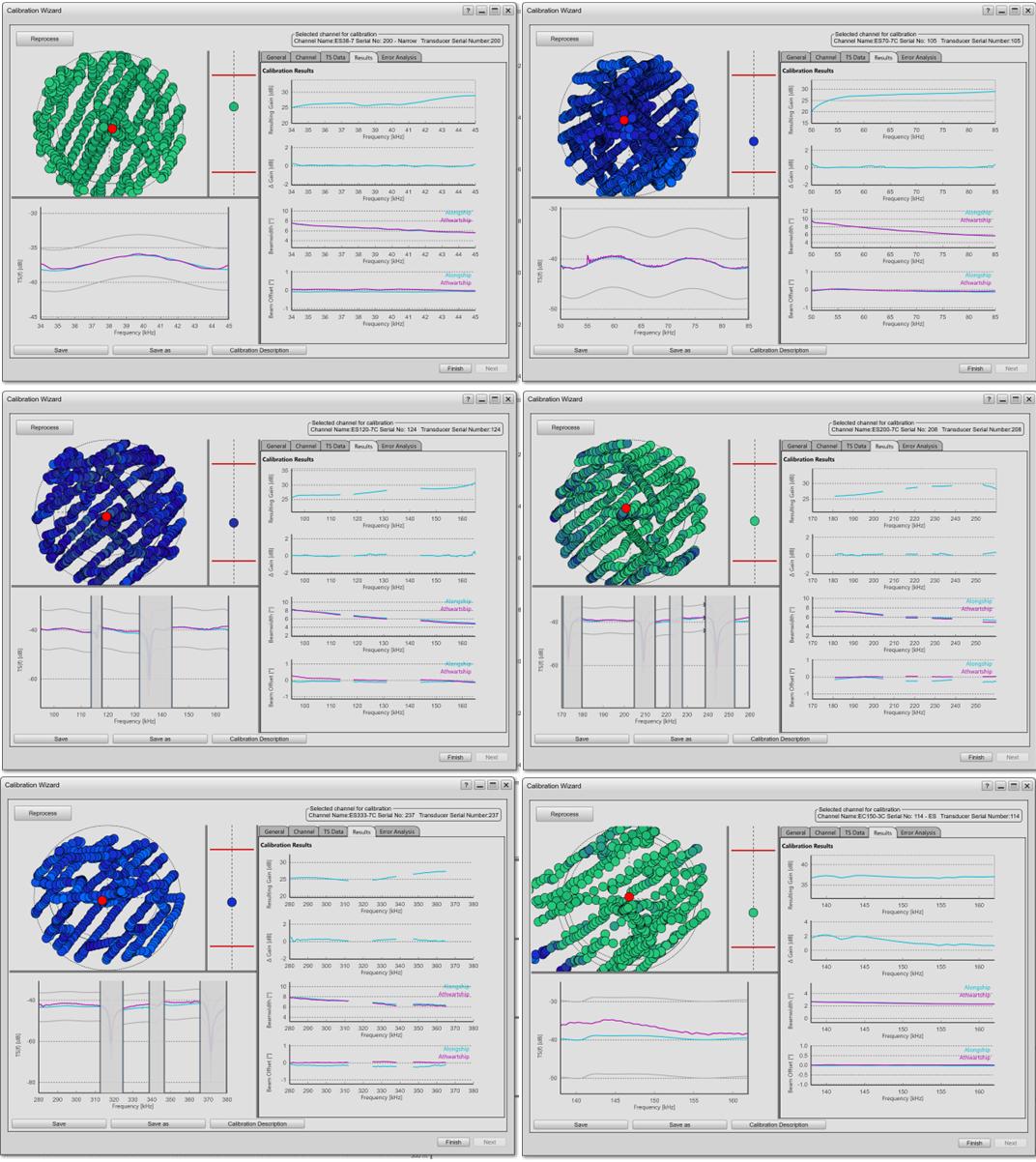
Ship drop-keel mounted echosounders (2022.11.27, Tromsø) were calibrated using standard (Demer, 2015) and metallic spheres of various sizes made of tungsten carbide with 6 percent cobalt binder. The calibration sphere diameter was chosen based on the best fit for the bandwidth in question in terms of the “null” positions in the frequency response of the sphere (Table 8 and Figure 15). Both narrowband and broadband pulses were calibrated; calibration data log in Table 9. Example calibration results are shown in Figure 16. A second calibration target of a different size was used where needed to ensure calibration data across the entire bandwidth of the chosen acoustic pulse and the two calibration results merged as per EK80 software procedures for it. Calibration target diameters used were 57.2 mm, 38.1 mm, 35 mm, 25 mm, 22 mm, and 20 mm, and these are referred to “WC” plus the diameter, e.g. WC38.1 (Table 9).
An additional weight (500g shackle) was used to stabilize spheres of smaller size (WC38.1, WC35, WC22, and WC20) when calibrating ship echosounders. It was suspended 5-7 m below the calibration target by 0.5 mm diameter nylon line. WC57.2 was used alone with no additional weights. All spheres had nylon line netting with 1-2 m long loop to ensure the calibration target is removed in range from the three winch-line suspension rig line and knot echoes that are present just above the calibration target.
Calibration conditions and quality were good to excellent. Calibration results text files (*.xml) may benefit from check-up and calibration re-run from acoustic raw data files before these are used to scale fish acoustic frequency response data.
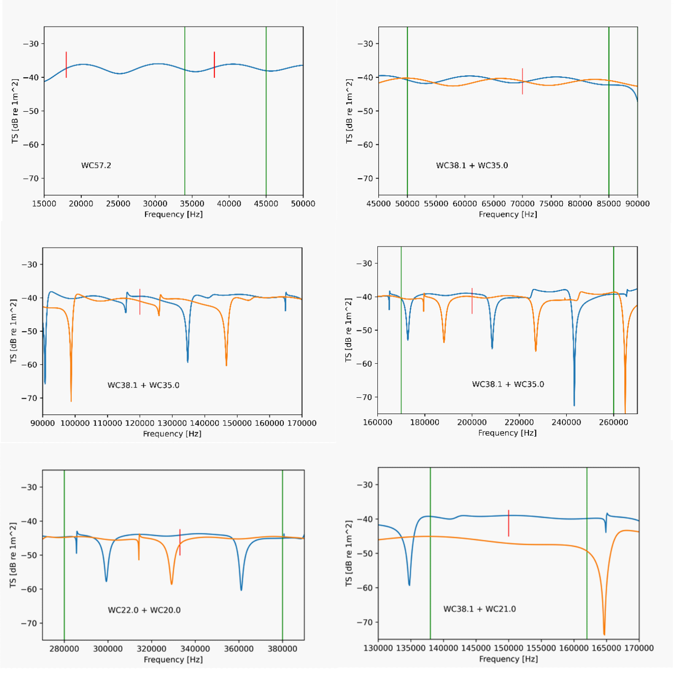
| 18CW | 38CW | 38FM | 70CW | 70FM | 120CW | 120FM | 200CW | 200FM | 333CW | 333FM | ||
| Sphere ID | BW (kHz) | - | - | 34-45 | - | 50-85 | - | 90-170 | - | 170-260 | - | 280-380 |
| IMR106 | WC57.2 | X | X | X | X | X | X | |||||
| IMR023 | WC38.1 | X | X | X | X | X | X | X | X | X | ||
| IMR123 | WC35 | X | X | X | ||||||||
| IMR139 | WC25 | X | X | X | X | |||||||
| IMR065 | WC22 | X | X | |||||||||
| IMR008 | WC20 | X |
| Chanel | Frequency [kHz] | Pulse shape | Pulse duration [ms] | Power [W] | Power taper | Beam mapping | Calibration target | EK80 Updated |
| 18-CW | 18 | CW | 1.024 | 800 | Fast | Full | WC57.2 | Yes, replace |
| 38-CW | 38 | CW | 1.024 | 400 | Fast | Full | WC57.2 | Yes, replace |
| 38-FM | 34-45 | FM-Up | 2.048 | 400 | Fast | Full | WC57.2 | Yes, replace |
| 70-CW | 70 | CW | 1.024 | 225 | Fast | Full | WC57.2 | No |
| 120-CW | 120 | CW | 1.024 | 100 | Fast | Full | WC57.2 | No |
| 200-CW | 200 | CW | 1.024 | 105 | Fast | Full | WC57.2 | No |
| 70-CW | 70 | CW | 1.024 | 225 | Fast | Full | WC38.1 | Yes, replace |
| 70-FM | 50-85 | FM-Up | 2.048 | 225 | Fast | Full | WC38.1 | Yes, replace |
| 120-CW | 120 | CW | 1.024 | 100 | Fast | Full | WC38.1 | Yes, replace |
| 120-FM | 95-165 | FM-Up | 4.096 | 100 | Fast | Full | WC38.1 | Yes, replace |
| 200-CW | 200 | CW | 1.024 | 105 | Fast | Full | WC38.1 | Yes, replace |
| 200-FM | 170-260 | FM-Up | 4.096 | 105 | Fast | Full | WC38.1 | Yes, replace |
| 333-FM | 280-380 | FM-Up | 4.096 | 40 | Fast | Full | WC38.1 | No |
| 38-FM | 34-45 | FM-Up | 2.048 | 400 | Fast | Full | WC38.1 | No |
| EC-150-3C | 150 | CW | 1.024 | 90 | Fast | Full | WC38.1 | Yes, replace |
| EC-150-3C | 138-162 | FM-Up | 2.048 | 90 | Fast | Full | WC38.1 | Yes, replace |
| 38-CW | 38 | CW | 1.024 | 400 | Fast | Full | WC38.1 | No |
| 120-FM | 95-165 | FM-Up | 4.096 | 100 | Fast | Full | WC35 | Yes, MERGE |
| 200-FM | 170-260 | FM-Up | 4.096 | 105 | Fast | Full | WC35 | Yes, MERGE |
| 333-FM | 280-380 | FM-Up | 4.096 | 40 | Fast | Full | WC35 | No |
| 200-FM | 170-260 | FM-Up | 4.096 | 105 | Fast | Full | WC25 | Yes, MERGE |
| 120-FM | 95-165 | FM-Up | 4.096 | 100 | Fast | Full | WC25 | No |
| 333-FM | 280-380 | FM-Up | 4.096 | 40 | Fast | Full | WC25 | No |
| 333-CW | 333 | CW | 1.024 | 40 | Fast | Full | WC25 | No |
| 333-CW | 333 | CW | 1.024 | 40 | Fast | Full | WC22 | Yes, replace |
| 333-FM | 280-380 | FM-Up | 4.096 | 40 | Fast | Full | WC22 | Yes, replace |
| 333-FM | 280-380 | FM-Up | 4.096 | 40 | Fast | Full | WC20 | Yes, MERGE |
| All CW in PASSIVE | CW | PASSIVE record. 200pings. 700m record range. Ping rate 1/sec. | ||||||
| All FM in PASSIVE | FM-Up | PASSIVE record. 200pings. 700m record range. Ping rate 1/sec. | ||||||
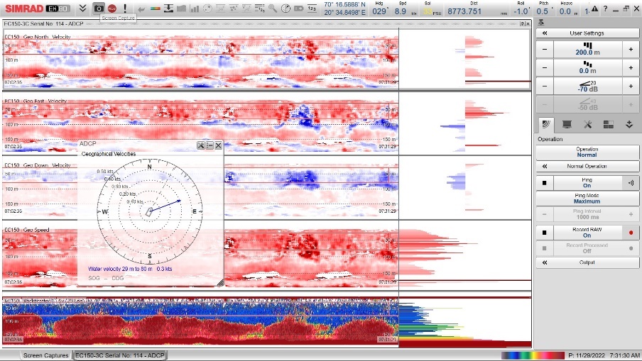
4.2 - Simrad EC150-3C ADCP calibration
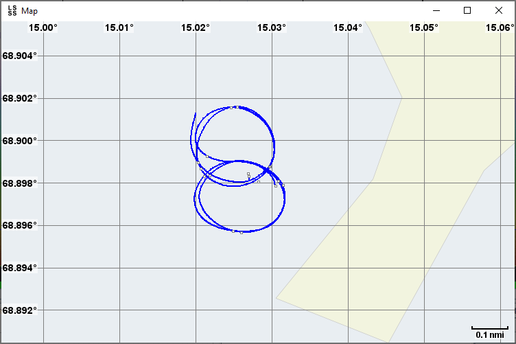
The Simrad EC150-3C ADCP / echosounder is installed on the ship drop-keel and is capable of CW and FM pulse generation both when operated as an ADCP and as a scientific fisheries echosounder of rather narrow beamwidth (2.5°) with both narrow- and broad-band acoustic pulses. It was calibrated with WC38.1. The ADCP beam was calibrated along with the other ship based echosounders, c.f. Table 8.
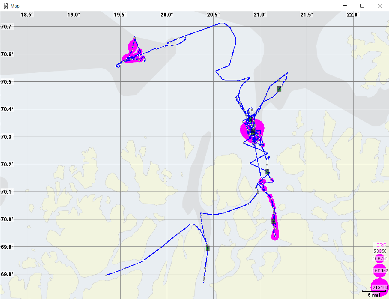
The Simrad EC150-3C ADCP calibration was performed in Kvænangen fjord, north of Tromsø (2022.11.29, 06:58-07:33) and in fjord outside Myre, Lofoten (20222.12.02, 11:04-11:34 UTC). A standard procedure was followed (provided by the producer). Ship sailed 2 circles clockwise and 2 circles anticlockwise at >6 knots speed (Figure 17). Circle diameter 200-400 m. Bottom depth approximately 200 m (Kvænangen) and 100m (Myre). Note that there was much herring in the water column in Kvænangen (Figure 18). Ample herring in the water column had no negative effect on ADCP calibration.
EC150-3C ADCP and RDI ADCP inter-calibration was performed close to Vestrålen (2022.12.02, 07:30-09:49 UTC). The two ADCP’s ran synchronised with each other. Vessel sailed at 10 knots for 1h west out of the fjords into the open sea, turned about and returned on the same path.
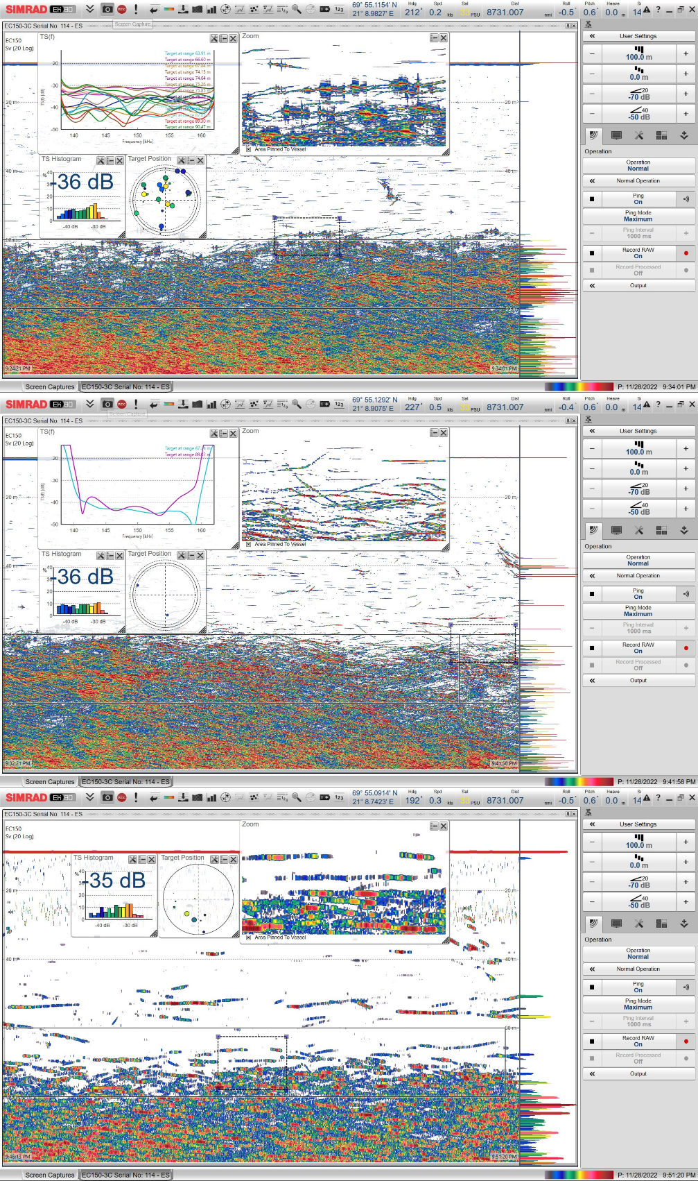
4.3 - EC150-3C operation as echosounder
Dataset was collected with EC150-3C unit operating as an echosounder of rather narrow, 2.5° beamwidth. Three setting were used: linear up-sweep, 138-162 kHz pulses of 2 ms duration with “fast” and “slow” taper, and 150 kHz narrowband pulses of 1 ms duration. The ability to resolve individual herring at the outskirts of a dense fish layer residing at 60-80 m depth was demonstrated (Figure 19). The Ship keel-mounted echosounders (7° beamwidth) were unable to resolve herring as individuals at this range. A 30 min long datasets were collected on 2022.11.28 21:35 UTC and 2022.11.29 19:50 UTC in Kvænangen fjord and in the open sea 12 nmi westwards of Kvænangen fjord, respectively.
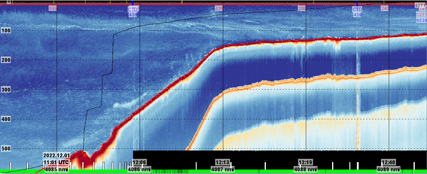
4.4 - Node 7 EK80 echosounder calibration
Objective
The objective of this task was to do broadband calibration of the seafloor mounted EK80 (LoVe Node 7) according to Ona et al. (2020).
Method and results
The bottom mounted Node 7 Simrad EK80 echosounder (single ES70-7CD transducer) was calibrated according to Ona et al. 2020 (Figure 20). Prior to the calibration a CTD cast was performed. Two calibration spheres (WC57.2 and WC35) were suspended 14 m and 7 m, respectively, below the CTD frame. A Ø0.6 mm nylon line was used to attach the spheres to the frame. The Node 7 echosounder beam has a diameter of about 25 m at the sea surface (220 m range to surface). Remote access (Screen Connect) to the LoVe server was used to visually follow the positioning and data collection from the seafloor echosounder. To aid in position the sphere the backscattering from the CTD frame was used. After positioning the CTD and spheres within the beam close to the surface, the CTD frame was lowered to 40 m depth. The DP system of GO Sars was used to position and move the spheres within the acoustic beam of the node echosounder. Once the LoVe Node beam had been located, the vessel locked to the exact position using its DP system and, thereafter, moved slowly and precisely to achieve the beam coverage required for calibration. The vessel’s 70-kHz echosounder was in passive mode during the calibration to observe the background noise and avoid interference with the observatory echosounder transmitting every 1 s. A standard full beam mapping calibration was achieved.
4.5 - Noise observations
Rolf Korneliussen (IMR)
Objective
The objective of this activity was to verify methods developed to estimate noise in broadband measurements (FM). Both narrowband frequency-dependent noise (1) as well as ambient noise visible in pulse-compressed data (2) is investigated. Furthermore, it is necessary to investigate if estimation of noise can be achieved while active pinging (3). The removal of frequency-dependent noise is needed if there is a strong band-limited component that would reduce the quality of a sub-band.
Method
Data were collected from EK80 during the following times to investigate tasks (1), (2) and (3): 2022.11.28 00:00:28 UTC – 2022.11.28 05:07:42 UTC (Passive FM data, 18 kHz CW active), 2022.11.29 23:04:33 UTC – 2022.11.30 14:27:13 UTC (Active FM data, 18 kHz CW active).
The measurement of narrowband frequency-dependent noise in FM (Task 1) were investigated by continuously measuring the local noise and comparing that to the local noise-floor. If the local noise was above a specified relative strength (here: 4 dB above the local noise-floor), it was registered as a noise-frequency. Furthermore, the width of the noise-peak was measured, defined as the width between the 50% level on both sides relative to the peak value. Then a gaussian distribution were used to estimate the width 90% down from the peak to get a measure of the width of the frequency-dependent noise-peak. The noise distribution may nort strictly follow a gaussian distribution as long as the noise has a gaussian distribution close to 90% upper part of the distribution.
The noise spikes are typically seen as vertical lines in the frequency domain (Figure 21). Removal of band-limited frequency-dependent noise use both frequency and bandwidth as input to a notch filter. The notch-filter is essentially a frequency-dependent multiplicator that dampen the signal at the noise-frequency and reduce the values at the neighboring frequencies according to an exponential function using a specified bandwidth.
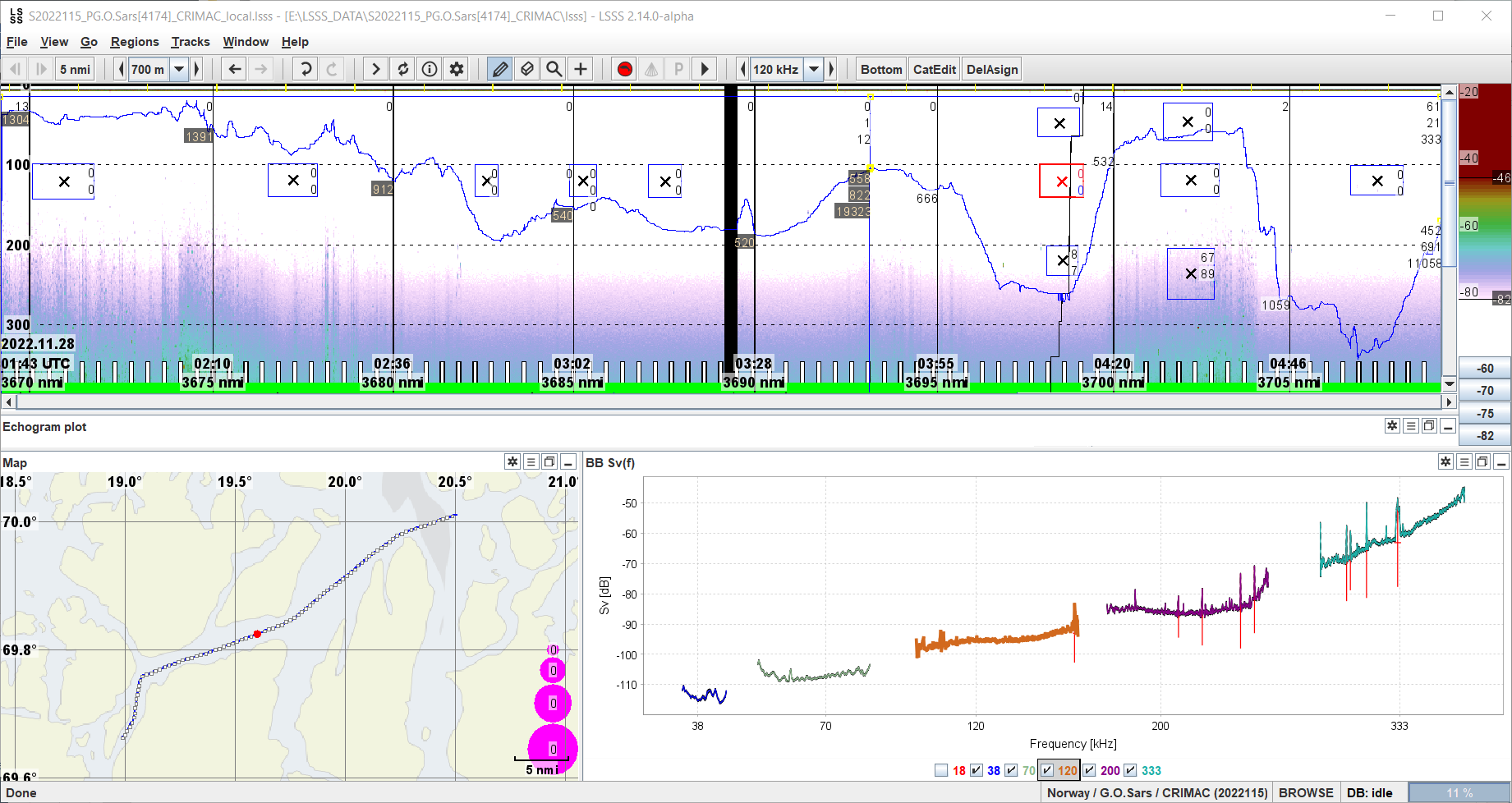
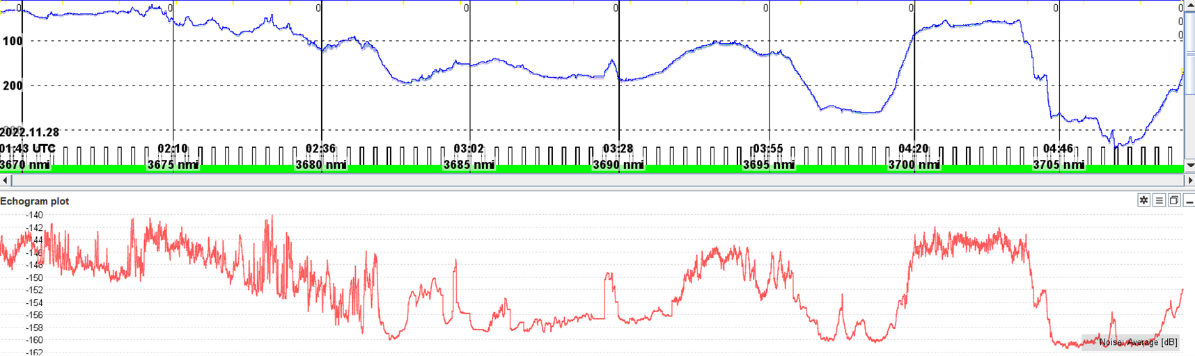
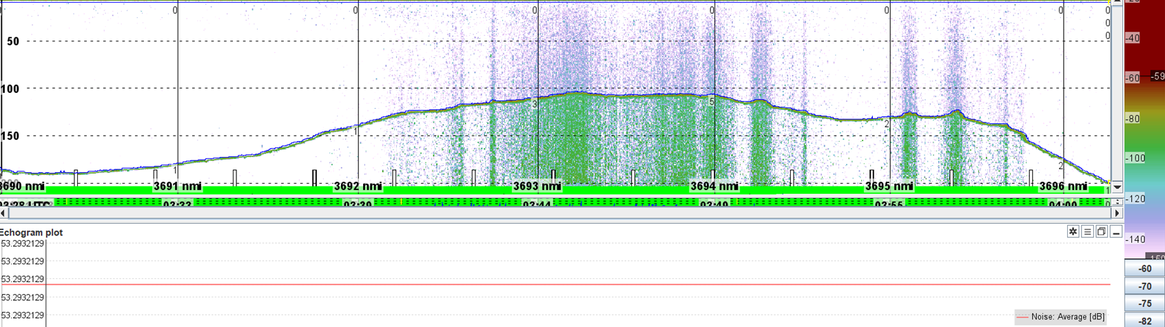
The ambient noise was also measured in passive pulse-compressed data (Task 2). All frequencies were run in FM mode using similar settings as during the calibration, except that they were all run in passive mode and that the 18 kHz CW channel were set to the minimum allowed power, i.e., 160 W instead of 800 W. The 18 kHz were operated in active model to measure bottom depth during recordings, and the low power were used to avoid interference with the other frequencies. The passive recordings were collected during bottom-depths varying from 30 m – 330 m. Figure 22 shows the bottom and the estimated noise at 38 kHz. Note that the noise is highly correlated with the bottom depth.
If we calculate a single value across the data set for 70 kHz (Figure 23) we obtain essentially the same results as for the 38kHz case(Figure 22), except that there is one value for noise as opposed to an estimate for all distances. The single noise-value is the 5% lowest value of noise at 70 kHz, and for most distances less noise is removed compared to the case where noise is estimated across all distances. Note that the Sv threshold of -150dB is far below the standard -82dB used in IMR surveys, and only very weak signal is affected by the noise removal. Note also that there are some vertical regions of weak signal that follows both the bottom depths and the bottom contour.
4.6 - FM to CW comparisons
Rolf Korneliussen (IMR)
Objective
To change data collection in acoustic trawl surveys from multiple frequencies (CW) to broadband, we need to verify that the methods to split broadband measurements into sub-bands to emulate CW signal produce comparable results. The broadband sub-bands are pulse-compressed and sometimes erroneously referred to as CW bands. It is essential that these provide the same results to maintain the time series for acoustic trawl surveys.
Method
To test if the method works it is essential with reliable calibrations. This was our first survey where the echosounders were calibrated at both the CW and FM settings to be used during the survey, except a small deviation in power setting to allow sequential pinging.
The EK80 mission-planner allowing advanced sequencing of different pulse types were used to alternate between CW and FM pinging. The power was deviating from the standard IMR settings allowing sequential pinging between the CW and FM settings, but different power were used at different channels following the power setting for the FM according to the IMR procedure. This was necessary according to the manufacturer (Simrad / Kongsberg) as the electronics (condensator) would not be able to recharge and empty when changing from a CW-ping to a FM-ping at a different power.
The data were first collected at maximum ping rate alternating between 2 pings in CW mode followed by 2 pings in FM mode. With these settings, the echosounder was unable to maintain maximum ping-rate and we experienced several lost pings. The ping-rate was reduced to one ping per 1500 ms, alternating between 1-ping-CW and 1-ping-FM. The sequence was easily identifiable in the data, but could suffer from the charge/recharge problem. To further investigate this, a more careful analysis will be needed.
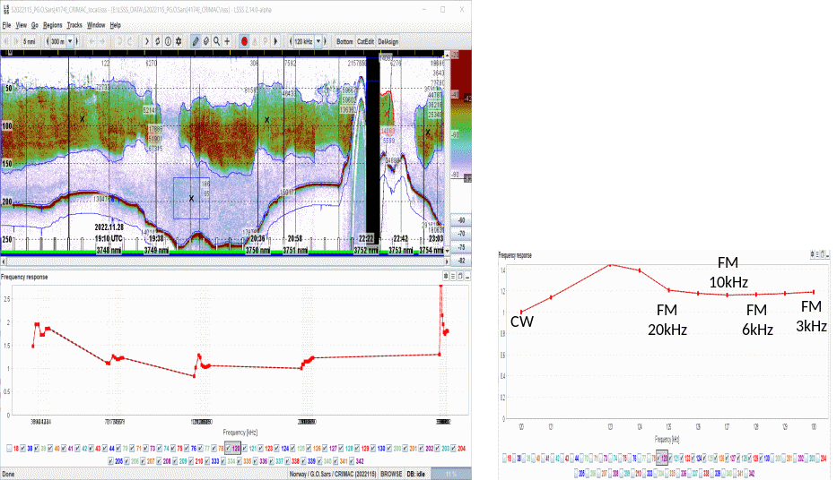
The test procedure is based on CW-data collected at a bandwidth close to 3 kHz in 1 ms pulses. The FM-data were collected by means of linear up-sweep FM. The bandwidth varied from 11 kHz (38 kHz channel) to 100 kHz (333 kHz channel) at either 2 ms (38 and 70 kHz) or 4 ms (120 – 333 kHz) channels. To compare the results, the summed CW for a school was compared with the FM bands for the same school with decreasing bandwidth (Figure 24).
4.7 - Remote acoustic sizing of herring
Babak Khodabandeloo and Rokas Kubilius (IMR)
Objective
The objective of this task was to size fish remotely by sideways-looking broadband acoustics. Two laterally sideways looking acoustic beams were used to inspect individual fish in situ at 25-150m range from the ship. These were a metal pole-mounted Simrad EK80 ES200-7C transducer and a modified MS70 processing setup where the array was used to generate a narrow split-beam instead of the full 3D ensonification.
Method
ES200-7CD pole-mounted, sideways-looking transducer
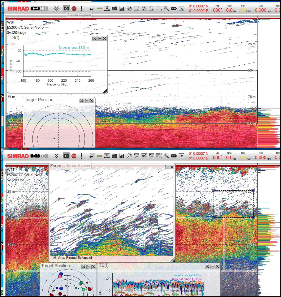
A single Simrad EK80 transducer (ES200-7CD, ID. 120) was mounted on a 7 m long metal pole installed on the starboard side of the mid-ship (Figure 25). The transducer was 2 m under the sea surface, tilted ~30° downwards. A 30 m long transducer cable allowed a dedicated Simrad EK80 transceiver to be placed in the ship hangar. The EK80 software were operated from a laptop in the ship instrument room via Ethernet communication. Echosounder was operated at 0.3 s-1 ping rate, producing 2 ms duration, up-sweep frequency modulated pulses of 160-260 kHz with “fast” or “slow” taper. Echosounder will be calibrated at the pier after the survey. The pole-mounted ES200-7CD transducer has a 7° nominal beam opening angle.
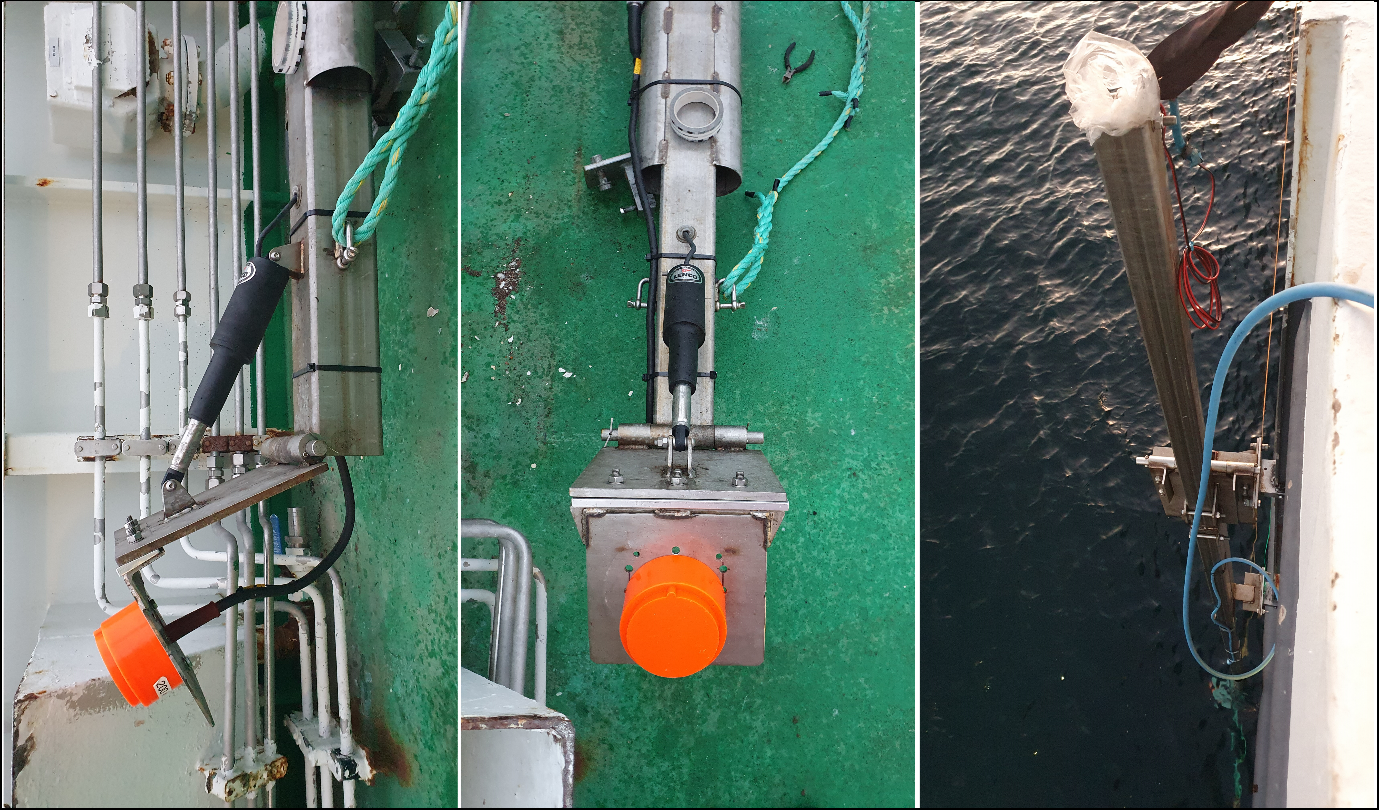
Pulse compression of broadband signal provides enhanced range resolution. The range resolution will be ~c/2B where c is the water sound speed and B is the bandwidth of the transmitted broadband signal. The transmitted pulses were 2 ms up-sweep linear frequency modulated 160-260 kHz, and the corresponding theoretical range resolution is ~7.5 mm. Data were collected by four different measurement configurations. Two different filter types, “standard resolution” and “short”, and two different tapers, “fast” and “slow”, were used. Four different setting configurations were used one at a time. Using filter type “Short”, the output file from EK80 has a slightly (~40%) higher sampling rate (or less decimation). Examples of echogram are shown in Figure 26.
MS70 setup with single, narrow beam
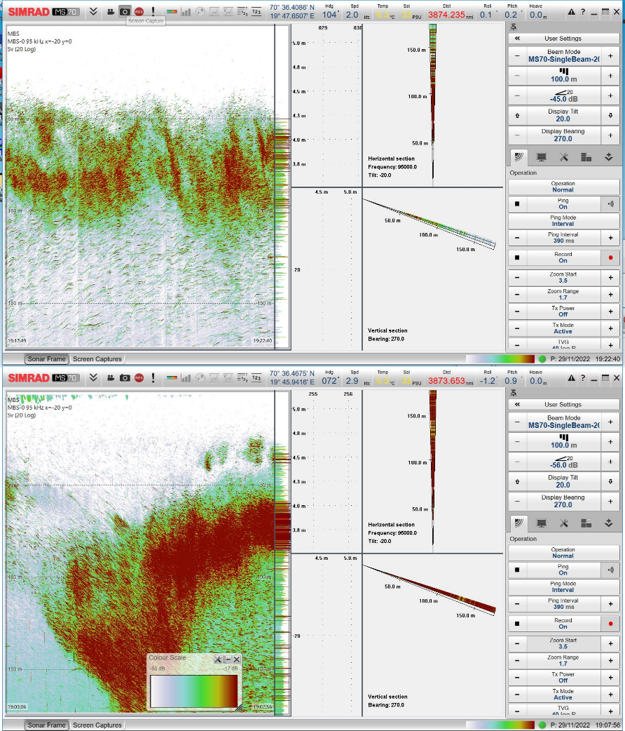
The MS70 scientific multibeam echosounder is installed on the ship drop-keel with transducer projecting sideways to the port side of the ship. A custom built MS70 software was used to generate a single narrow acoustic beam (5.9° tall, 3.4° wide) that could be steered vertically to 0, 5, 10, 15, or 20° tilt downwards. The 20° tilt was used on this survey. MS70 was operated with linear up-sweep, 70-120 kHz pulses of “slow” taper (as the only available setting option at the time). A comparatively narrower MS70 beam allowed for individual fish to be resolved at longer range as compared to ES200-7C system. Two snapshot echograms are shown in Figure 27.
Biological sampling
Biological samples were collected by trawling and fish length, weight, width, and height were measured for subsample of 100-200 fish. The measurement board was used to measure the length and weight, and these data are available through the NMBbiotic database. A digital calliper was used to measure the width and height, and the ID column can be used to combine the data with the length measurements. The height and width measurements are available in an excel sheet located at S2022115_PGOSARS_4174\BIOLOGY\CATCH_MEASUREMENTS\
The first data were collected from 28.11.2022 12:00 UTC to 29.11.2022 01:00 UTC (Kvænangen fjord). A second data set were collected in the open sea (about 12 nmi west of Kvænangen), from 29.11.2022 17:15 UTC to 20:20 UTC.
Preliminary results
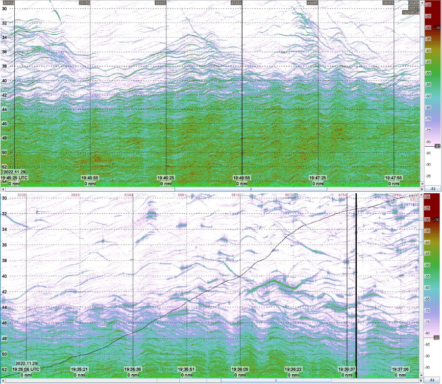
The pole-mounted ES200-7CD transducer/echosounder was able to resolve individual fish at 25-50 m range but not at 80 m range to fish (Figure 26). The MS70 single beam setup had a narrower beamwidth and was able to resolve fish at greater distance as compared to ES200-7CD (Figure 27). The slow taper pulses had less “temporal sidelobes” before and after individual fish echo detection as compared to fast taper pulse echo data (Figure 28).
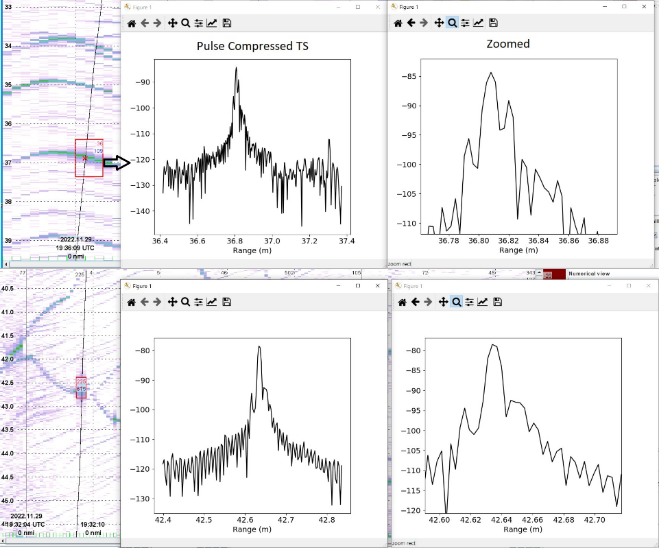
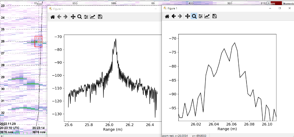
The initial processing of time-domain signals from ES200-7CD demonstrated muti-peak echo structure that appears to correspond well with the fish body width measurements from the trawl samples (approx. 3 cm, Figure 29). An attempt was also made to size fish body height using the vertically down oriented, ship drop-keel mounted ES200-7C transducer data (Figure 30). The height of the selected fish is approximated to be ~4-5 cm which agrees with the fish height measurements from the associated trawl catch.
4.8 - LoVe transect
Geir Pedersen (IMR)
Objective
The objective of this task was to 1) perform the standard IMR transect across the LoVe Ocean Observatory. The transect is covered four times per year and includes echosounding, ADCP, and CTD. An additional objective was to visually characterize the scattering layer across the transect using the Deep Vision system.
Method
The LoVe transect was performed from station 1 to station 6 (30.11.2022) with
a. Echosounders running standard IMR broadband settings and RDI long and short range ADCP
b. Deep Vision, which was deployed (IMR VITO pelagic sampling trawl) throughout the transect with a nascent/descent speed of approxiately 10-15 m/min covering surface to seafloor (as close as practical). From station 5 Deep Vision profiled 0-500 m. Deep Vision was deployed twice it two five-hour sessions with battery swap.
The LoVe transect was performed from station 6 to station 1 (01.12.2022) with
c. echosounders running standard IMR broadband settings
d. CTD casts from surface to seafloor at stations 6-1
Table 10. Description of the standard transect and sampling procedures (in Norwegian).
The westward transect was covered at vessel speed at three knots, with Deep Vision performing a V-shaped coverage of the water column (ascent/decent approximately 10 m/min), EK80 and ADCP data were collected concurrently with the Deep Vision data. The eastward transect was performed at normal survey speed at approximately 10 knots, with CTD stations along the transect (stations 6-1) as described in Table 10. Broadband acoustic data was collected according to the standard IMR settings as well as ocean current measurements (ADCPs). The cable transect and acoustic vessel transect are shown in Figure 31.

Preliminary results
The standard transect was successfully completed twice providing data to IMR LoVe time series database and CRIMAC (Figure 32). The first transect collected echosounder, ADCP and biological data (DeepVision). Figure 33 shows the path of the Deep Vision and example images.
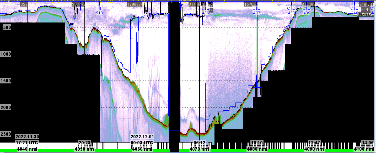
The data will be used to characterize dominant scattering layers at LoVe using broadband (EK80) and imaging (DeepVision). Further we will explore the capabilities of LoVe (discrete nodes with single frequency echosounder) to characterize these layers. Additional related questions are i) what the difference in is characterization power of LoVe and research vessel, do we observe the same (LoVe, Vessel, Deep Vision)?, ii) at what range from the nodes along the transects does the nodes provide “representative” observations?, iii) how representative are vessel observations at LoVe, vessel “snapshot” vs LoVe time series?
The second completion of the LoVe transect (Stations 6-1) consisted of broadband acoustic data collection with CTD and water sampling at the six stations (Figure 32, Figure 34). The acoustic and water column data will be used to investigate the capabilities of broadband acoustics to characterise the physical properties of the water column.
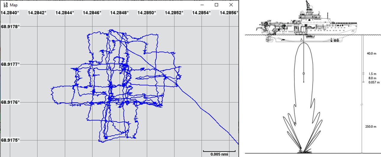
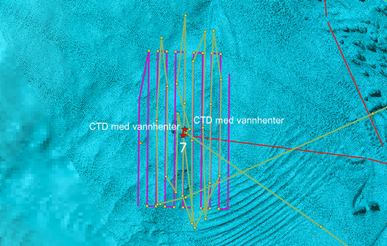
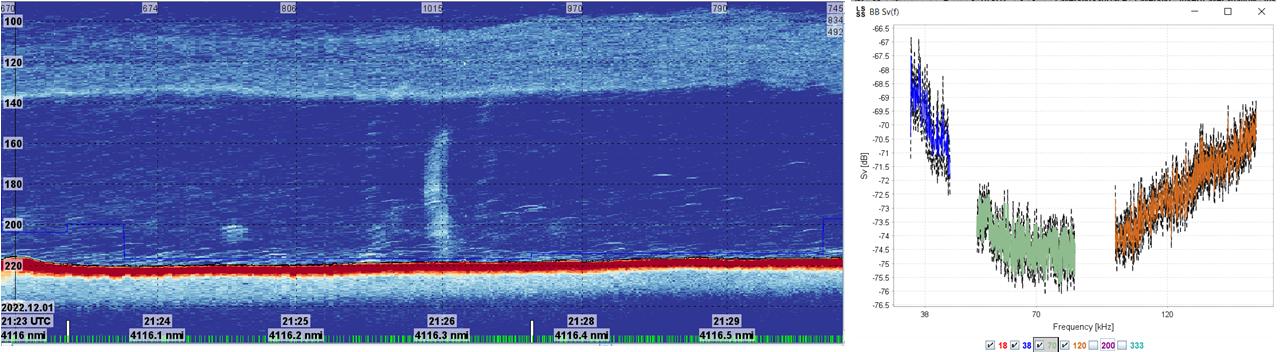
4.9 - Broadband gas seep detection and quantification
Geir Pedersen (IMR)
Objective
Known methane seeps are located around LoVe Node 7, and the objective of this task was to collect broad banded echosounder data of natural methane seeps.
Method
A survey grid was laid out covering Node 7 (Figure 35). GO Sars collected broadband data from both the EK80 and EC150. When plumes were located (e.g. close to Node 7) the plume was investigated further by placing the ship on top of the seep and collecting additional broadband echosounder (EK80) and ADCP (EC150) data (Figure 36).
The data will be scrutinized in the CRIMAC task on quantification of gas seeps, using this as an additional data set for testing methods for broadband characterization of methane seep using vessel and observatory based broadband acoustics (GO Sars broadband data, LoVe broadband data (70kHz), single bubble/aggregation models), and vessel based ADCP with narrowbeam vertical echosounder (EC150).
5 - References
Allken, V., Handegard, N.O., Rosen, S., Schreyeck, T., Mahiout, T., Malde, K., 2019. Fish species identification using a convolutional neural network trained on synthetic data. ICES Journal of Marine Science 76, 342–349. https://doi.org/10.1093/icesjms/fsy147
Demer, D. 2015. Calibration of acoustic instruments. ICES Cooperative research report No.326, International Council for Exploration of the Sea.
Korneliussen, R. J., Diner, N., Ona, E., Berger, L., and Fernandes, P. G. 2008. Proposals for the collection of multifrequency acoustic data. ICES Journal of Marine Science, 65: 982–994.
Ona, E., Zhang, G., Pedersen, G., and Johnsen, E. 2020. In situ calibration of observatory broadband echosounders. ICES Journal of Marine Science, 77: 2954–2959.
6 - Data organization
The data are organized in accordance with the IMR data organization procedure. In this section the placement of additional, non-standard, data sets are described.
ACOUSTIC
Data locations for ship EK80 and EC150-3C ADCP / echosounder calibrations:
S2022115_PGOSARS_4174\ACOUSTIC\EK80\EK80_CALIBRATION
S2022115_PGOSARS_4174\PHYSICS\ADCP\ES150_KHZ
OBSERVATION PLATFORMS
S2022115_PGOSARS_4174\OBSERVATION_PLATFORMS\POLEMOUNTEDEK80
This is the location for the pole mounted EK80 data.
S2022115_PGOSARS_4174\OBSERVATION_PLATFORMS\FOCUS2
This is the location for the data collected with the towed underwater vehicle (FOCUS) with the following subfolders: VIDEO (FOCUS camera) and MESOTECH (scanning sonar) with an additional subfolder for each trawl haul (496 and 502).
S2022115_PGOSARS_4174\OBSERVATION_PLATFORMS\WBAT \WBAT_EK80_RAWDATA
This is the location for the raw data from WBAT attached in the trawl. Subfolders for each trawl haul.The mission plans and a description of how the wbat was mounted in the trawl are also stored in this location.
BIOLOGY
S2022115_PGOSARS_4174\BIOLOGY\CATCH_MEASUREMENTS\
This is the location for the biological data related to the acoustic length measurements (23307, 23307 and 23308), where also the height and width of the fish were measured. The data is recorded in the file:
S2022115CRIMAC_widthandheightmeasurements.xlsx
with an ID field that corresponds to the ID field in the NMDbiotic database.
S2021111_PGOSARS_4174\BIOLOGY\CATCH_MEASUREMENTS\OTHER_MULTIMEDIA\GOPRO_TRAWL
GOPRO videos from trawl are stored in this location. Subfolder for each trawl haul including description of placement
S2022115_PGOSARS_4174\BIOLOGY\CATCH_MEASUREMENTS\OTHER_MULTIMEDIA\DARKVISION CAMERA
Darkvision camera attached opposite to wbat in trawl videos are stored in this location. Subfolder for each trawl haul. Data have been processed using videoprostprocessing.py
S2022115_PGOSARS_4174\BIOLOGY\CATCH_MEASUREMENTS\DEEP_VISION
Deep Vision data are stored in this location. Subfolder for each trawl haul (Deep Vision session, date and time when logging started)
S2022115_PGOSARS_4174\BIOLOGY\TRAWL_SENSORS\SCANMAR
Trawl sensor data are stored in this location. Scanmar data were collected and stored both from the “old” SCANBAS system and the “new” Scanmar 365 system. Continuous nmea strings were extracted from both systems as well as datafiles corresponding to each station. For the “old” system station data are also parsed into tab and semicolon delimited files.
“ OLD” SCANBAS system
S2022115_PGOSARS_4174\BIOLOGY\TRAWL_SENSORS\SCANMAR\Scanbas
“ New” Scanmar 365 system
S2022115_PGOSARS_4174\BIOLOGY\TRAWL_SENSORS\SCANMAR\Scanmar_365
S2022115_PGOSARS_4174\EXPERIMENTS\GPS_GPX
GPS log (.gpx files with fix every second, only leg 1 of cruise).
These files can be used to quickly find location at any time during leg 1 of the cruise (22-26.11). They were collected using Shale’s private GPS unit (Garmin GPSmap 60CSx). The GPS unit turned itself off from 00:00:00-10:12:30 on 25.11, so no fixes are available during that time period.