Report series:
Toktrapport 2025-7ISSN: 1503-6294Published: 08.05.2025Project No.: 15925On request by: Institute of Marine Research Approved by:
Research Director(s):
Geir Huse
Program leader(s):
Henning Wehde
Dette toktet hadde som mål å studere mulige miljøeffektene av flytende havvind installasjoner, med fokus på marine økosystemer. Dataene som ble samlet inn under dette toktet er viktige, ettersom det er begrenset kunnskap om hvordan denne teknologien påvirker miljøet. Toktet er en del av Havforskningsinstituttets havvind forskning, og er en oppfølging av studier gjennomført i 2023 og med planer om tilsvarende studier for 2025. Dette toktet bidrar også med data til to forskningsprosjekter: WINDSYS (Norges Forskningsråd), som undersøker effekten av vindfarmene på pelagisk fisk, og ORCHESTRA (JPI Oceans), som studerer effekten av konstant undervannsstøy på zooplankton.
I 2023 gjennomførte vi en rekke akustiske transekter med G.O. Sars rundt vindparken, men med mindre tid tilgjengelig måtte vi redusere antall transekter. For å undersøke hvilke arter som er til stede og distribusjon av disse ble det også brukt en trål med kamera (DeepVision) og miljøprøvetaking (eDNA). I tillegg ble det plassert en FAD (Fish Aggregation Device) inne i vindpark området, utstyrt med bl.a. hydrofon, miljøsensorer og ekkolodd, denne håper vi skal tiltrekke seg pelagisk fisk slik at vi kan studere effektene av støy fra vindturbinene på fiskens atferd. En bunn montert instrument rigg (Lander), også den utstyrt med hydrofoner, ekkolodd og miljøsensorer har stått i parken siden februar 2024 for å overvåke fiskens atferd relater til lyd og miljøfaktorer, på toktet hentet vi denne lastet ned data og plasserte den ut igjen. Videre ønsket vi å undersøke virkningen av den flytende havvind installasjonen på de oseanografiske forholdene (vannets lagdeling og turbulens) og planktonfordeling ved hjelp av en rekke CTD transekter med bruk av plamkton nett og MICRO-CTD for mer detaljerte målinger. Det dårlige været førte til at bare to av i alt 14 planlagte MICRO-CTD stasjoner og fire CTD stasjoner ble gjennomført. Vi prioriterte den tilgjengelige tiden på Hywind Tampen (25 timer) på å få ut FAD og inn og ut Lander.
ORCHESTRA-prosjektet fokuserte bl.a. på hvordan støy fra vindparker påvirker zooplankton, spesielt copepoder. Det ble brukt bur med fri svømmerne copepoder, utstyrt med 3D kamerasystem og hydrofoner for å studere svømmeatferden relatert til støy. RNA-prøver ble tatt fra eksponerte og ikke-eksponerte copepoder. Pga dårlig vær ble dette studiet gjennomført i Sognefjorden og da med støy fra forskningsfartøyet og ikke på Hywind Tampen med turbin-støy som planlagt. To fugleobservatører var til stede under dagtid for å overvåke fuglelivet i området.
Summary
This expedition aimed to study potential environmental effects of an floating offshore wind installations, with a focus on marine ecosystems. Data collected during this expedition is important, as there is limited knowledge about how this technology may impacts the environment. The expedition is part of the Institute of Marine Research's offshore wind research and serves as a follow-up to studies conducted in 2023, with similar studies planned for 2025. It also contributes data to two research projects: WINDSYS (Research Council of Norway), which examines the effects of wind farms on pelagic fish, and ORCHESTRA (JPI Oceans), which studies the impact of continuous underwater noise on zooplankton.
In 2023, we conducted a series of acoustic transects with RV G.O. Sars around the wind farm, but due to limited time we had to reduce the number of transects. To investigate which species were present and their distribution, we also used a trawl with a camera (DeepVision) and environmental sampling (eDNA). In addition, a FAD (Fish Aggregation Device) was deployed within the wind farm area, equipped with, a hydrophone, environmental sensors, and an echo sounders. We hope this will attract pelagic fish, and by that allowing us to study the effects of turbine noise on their behavior. A bottom-mounted instrument rig (Lander), also equipped with hydrophones, echo sounders, and environmental sensors, has been in the park since February 2024 to monitor fish behavior in relation to sound and environmental factors. During the expedition, we retrieved the Lander, downloaded data, and redeployed it.
Furthermore, we aimed to investigate the impact of the floating offshore wind installation on oceanographic conditions (water stratification and turbulence) and plankton distribution using a series of CTD transects, including plankton net hauls and a MICRO-CTD for more detailed turbulence measurements. Due to bad weather, only two out of the 14 planed MICRO-CTD stations and four of the CTD stations were completed. This as we prioritized the available 25 hours at Hywind Tampen to deploy the FAD and to retrieve and redeploy the Lander.
The ORCHESTRA project focused, among other things, on how noise from wind farms affects zooplankton, particularly copepods. Cages with freely swimming copepods, equipped with a 3D camera system and hydrophones, were used to study swimming behavior in relation to noise. RNA samples were taken from exposed and non-exposed copepods. Due to bad weather, this study was conducted in the Sognefjord using noise from the research vessel instead of at Hywind Tampen with turbine noise as originally planned. Two bird observers were present during the daytime to monitor bird life in the area.
1 - Background
1. Hywind Tampen windfarm
Hywind Tampen (HT) is the first offshore windfarm in Norwegian waters and probably the biggest floating wind farm in the world at the moment. It is built and operated by Equinor and supports oil and gas installation Gullfaks and Snorre with renewable energy. It was constructed during 2022-2023 and holds 11 turbines with a total capacity of 88 MW. For more details on Hywind Tampen, structure and design look at (rapport Equinor, 2019).
2. Aim of cruise
There is little knowledge related to how floating wind farms effect the marine environment, as this technology is still relatively new. Thus, data gathered on this cruise is noel in that sense. The aim of the cruise was to follow up studies done during a cruise in 2023 (Utne-Palm et al. 2023) our first cruise to HT, looking at possible environmental effects on the marine environment. This year, however, we had only one week compared to 13 days last year. We therefore prioritized topics and tasks that we have promised to look at in ongoing research projects. 1) WindSys “Effects of floating wind farms on the marine ecosystem, with a focus on pelagic fish” a cross disciplinary project funded by the Norwegian Research Council (336334). 2) Orchestra "ecOsystem Responses to Constant offsHorE Sound specTRA” a JPI Oceans project (339519).
WindSys focuses on the effect of HT on pelagic fish behaviour and distribution. Thus, to look at possible effects on pelagic fish distribution, we conducted several acoustics transects through and around the wind farm with RV G.O. Sars last year (Utne-Palm et al. 2023). With only half the time available this year, we decided to cut down on transects. We aimed to complete the transect straight through HT and the flower like transect around HT. For ground truthing of acoustic findings we also this year used a trawl with an open cod-end equipped with a camera (DeepVision) and we took eDNA samples.
Reef effect: G.O. Sars is not allowed closer then 500m to the turbines, thus, in 2023 we used an acoustic kayak-drone within the 500 m range to the wind turbines. With the kayak drone we managed to get as close as ca 20 m to the turbines, however, this was not close enough to see the fundament and the area close by where we expect to find fish aggregations (Reef effect). On this cruise we used the research vessels sonar MS70 multibeam sonar hoping would reach the 500 m to the turbine. As part of WindSys project we also deployed an ObsFAD (an observation station including a Fish Aggregation Device) at HT, holding an echosounder and a hydrophone. Hopefully this device will aggregate pelagic fish, and allow behavioural studies related to the temporal variations in windfarm noise. As part of the WindSys project, where Equinor is a collaborator, we also have a Lander at HT. This lander was deployed by, Equinor, in February 2023, and it holds, a bottom mounted multibeam echosounder, ADCP, hydrophones, CTD, oxygen – and turbidity sensors. Thus, the Lander will give us the possibility to observe fish behaviour related to sound and other environmental factors. During the cruise, we aimed to download the data from the lander and re-deploy it.
Orchestra’s research focus is on the effect of continuous underwater noise on invertebrates, with a focus on zooplankton (copepods) at HT during this cruise. Our aim was to test in-situ wether noise from an offshore wind farm (OWF) would affect zooplanktons swimming behaviour or RNA expression. To study swimming behaviour we use a free drifting cage set-up, holding free swimming copepods. The cage set-up was equipped with 3D camera and hydrophones, to enable comparison between copepods and in-situ noise. RNA samples will be taken from nonexposed copepods and exposed copepods (inside and outside the park) and before and after been exposed in the cage experiment. Further, we planned to look at how the wind wake effect water stratification, current and plankton distribution. For this we plan to do transects across the windfarm and shelf area, with 12 CTD stations. Each station included water-bottle samples for nutrients, plankton community and eDNA. For a more detailed resolution of the turbulence in the water column, we planned to use a MICRO-CTD, from now on referred to as MSS probe, on the CTD stations that were outside the 500 m safety zone.
Two bird observers were on deck during daylight hours when we had the wind farm in sight.
2 - Activity
2.1. At Hywind Tampen(20th of October and 25th to 26th of October 2024)
A detailed logbook of all activities during the cruise is available in Appendix (7.1. Cruise Timeline).
Given bad weather predictions, with only a narrow window of 7 to 8 hours of less strong winds, over the next 4-5 days, we steamed directly to Tampen, skipping the pre-testing of new and novel equipment in the fjord.
Priority 1 on for our cruise was to deploy a Fish Aggregation Device (FAD) at Hywind Tampen (HT), and to retrieve a Lander that have been logging data at HT, downloading its data and redeploy it after recharging the battery for the echosounder.
2.1.1. FAD
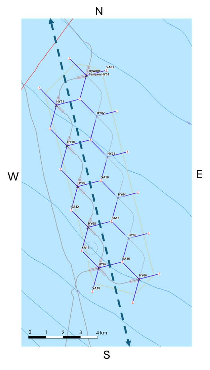
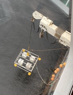
Before entering Hywind Tampen we contacted Equinor to open our working licences at HT. We started with deploying the FAD (Fish Aggregation Device) as it is a smaller task than bringing in the Lander. We deployed the FAD in position N61° 18,685, E002° 15, 576 (degrees min and sec). The aim was to place these to device in the vicinity of each other, so that if the FAD attracts fish, the sensors on the Lander will also gather data that is relevant for the observed behaviour at the FAD. Thus, Lander and FAD were placed in the same zone between Hywind Turbine 7 and 8 (HY08 and HY07, orange circle in Figure 3).
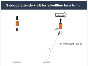
With its ensemble of buoys, the FAD is meant to attract fish (10 Vitrovex spheres, at ca 30 m depth). If it works as a FAD, our aim is to study the behaviour of the aggregated fish in relation to the noise and environmental data - using echosounders data in comparison with hydrophone and CTD data, as well as potential interactions with diving birds. The FAD also holds a telemetry receiver, to register marked fish or mammal passing the HT area. The battery and memory storage on the FAD will lasts for ca 5 months (same deployment time as the Lander, due to same type of instruments). The FAD would log data until April 2025.
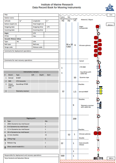
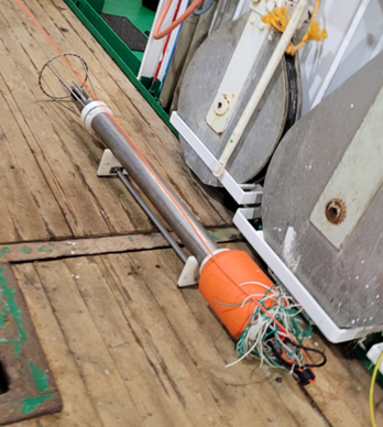
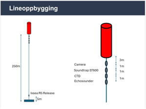
FAD details: The moorings consist 10 Vitrovex spheres attached by Dyneema rope to an acoustic release which is attached by chain to a bottom anchor in form of train wheels. A hydrophone (Soundtrap ST500), WBAT (Wide Band Autonomous Transceiver) Simrad, with two broadband transducers, Simrad ES70-18CD split-beam transducer and Simrad ES ES200-7CD split-beam transducer and batteries, a CTD (RBR Concerto) and telemetry receiver (Innovasea VR2W) are all added to the moorings by clamping onto the rope below the FAD (10 Vitrovex spheres) see Figure 1.
The FAD mooring construction has been evaluated by Delmar, to make shore that the buoyancy, weight and wire was strong enough to manage extreme weather (see Appendix 7.2).
Retrieving the FAD: the FAD is retrieved by triggering the acoustic release connected to the bottom anchor.
Figure 1. Drawing of an FAD (Fish Aggregation Devise) mooring and instrument information. Drawing by T. Hovland and S. Menze.
2.1.2. Lander
After having safely deployed the FAD, we released the Lander, using the Landers built in acoustic release system. It came quickly to surface and was easy to spot when at surface, due to its bright yellow colour.
The Lander with its many sensors (se Figure 2), is used to give us a point measure of temporal variations in environmental conditions and fish activity at HT. This is valuable information in particular when seen in connection with spatial data from the yearly cruises.
The lander was deployed in February 2024. The mission on this cruise was to retrieve it, download data and recharge batteries, before deploying it again in the same position. After downloading the data, we found that the Recordings started – 19.02.2024 at 07:00 and stopped on the – 22.07.2024 at 17:00. There was also an Around system freeze period between 12.03.2024 and 30.03.2024. Thus, the Lander will log data until April 2025.
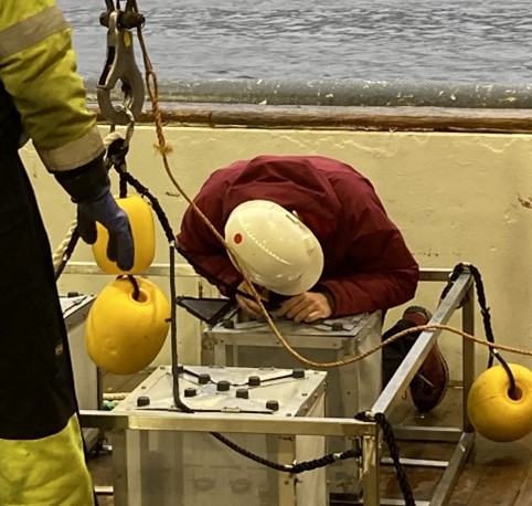
We had two people from Develogic onboard the vessel to handle the Lander and to train IMR personal in the use of this device. The Develogic Release system allows remote triggered recovery of the Lander without the need of subsea operations. However, the Lander is equipped with an ROV hook for pick-up. The original plan was to use an ROV pick up the lander, however, we decided to exclude the ROV to save money. Thus, to pick up the Lander we needed to get a rope through the ROV hook (~10 cm Ø) and connect the rope to the vessels winch. This was an incredible difficult task from deck, with the tiny opening, and a swell of 2-3 m. But, thanks to a smart and creative deck crew we managed to get a rope through the ROV hock and on to the winch. After retrieval, we added a cable loop with buoys to the Landers ROV hook, to make the next retrieval easier.
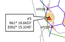
One of the three hydrophones broke during the struggle getting the Lander on board. However, the Lander data was all intact except for some issue with the CTD data. The lander was recharged and checked by the Develogic team on board. It was deployed on the last day of the cruise (25th of October at 18 o’clock) in the very same spot, between HY08 and HY07, in position N 61°18.6653ˈ, E002°15.3245ˈ (Figure 3). The HIPAP system was used for the positioning it during deployment. Unfortunately, G.O. Sars HIPAP system did not work, so the position is not 100% sure.
Unfortunately, was it not possible to repair the broken hydrophone during the cruise, and it looked like the lander was not logging CTD data after deployment.
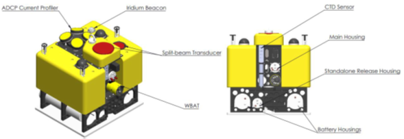
Lander detail: is built by Develogic. It holds three hydrophones type HTI-99 UHF, ADCP (Acoustic Doppler Current Profiler) Nortek Signature100, CTD (Conductivity, Temperature and Depth) Seabird SBE37-SMP MicroCAT, oxygen sensor (Aanderaa Oxygen Optode 4330) and transmissometer, , WBAT (Wide Band Autonomous Transceiver) Simrad, with two T218 transducers, Simrad ES70-7CD split-beam transducer and Simrad ES120-7CD split-beam transducer, data logging system and batteries.
Retrieving the Lander: The Lander housing (in titanium) is connected to a steel platform that functions as a weight. The Lander holds a built-in acoustic release system, that releases the Lander from its platform. A connection wire between the Lander and the platform makes it possible to pick up the entire device without using an ROV.
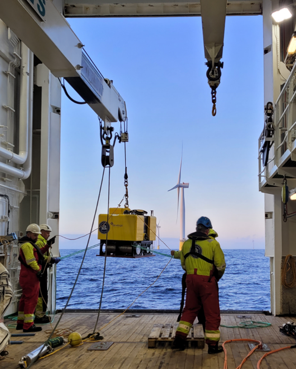
Figure 2. Deploying the Lander (top). Picture by K. de Jong. Lander with main components (bottom). Picture from Lander manual.Figure 3. Position of Lander at Hywind Tampen, depth is 280 m. The ObsFAD was placed at N61° 18,685, E002° 15, 576 (degrees min and sec), within the same area (orange circle) as the Lander.
2.1.3. Circulation patterns in and around Hywind Tampen
Our aim was to investigate the impact of the modification of the wind field by wind energy extraction (Wake effect) on ocean current speed and direction and potential implications for up- and downwelling. This is highly relevant for distribution of nutrients and planktonic organisms which form the base of the marine ecosystem. Ideally, we aimed at deploying an array of bottom-anchored ADCP moorings in and around the wind park to collect observations of upper ocean currents in the area, like we did on last year’s cruise (Utne-Palm, 2023), but as we only got 7 of the 14 days we applied for, this cruise did not allow time that type of sampling.
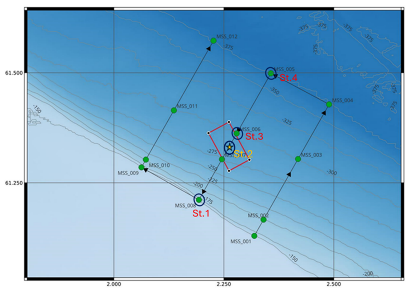
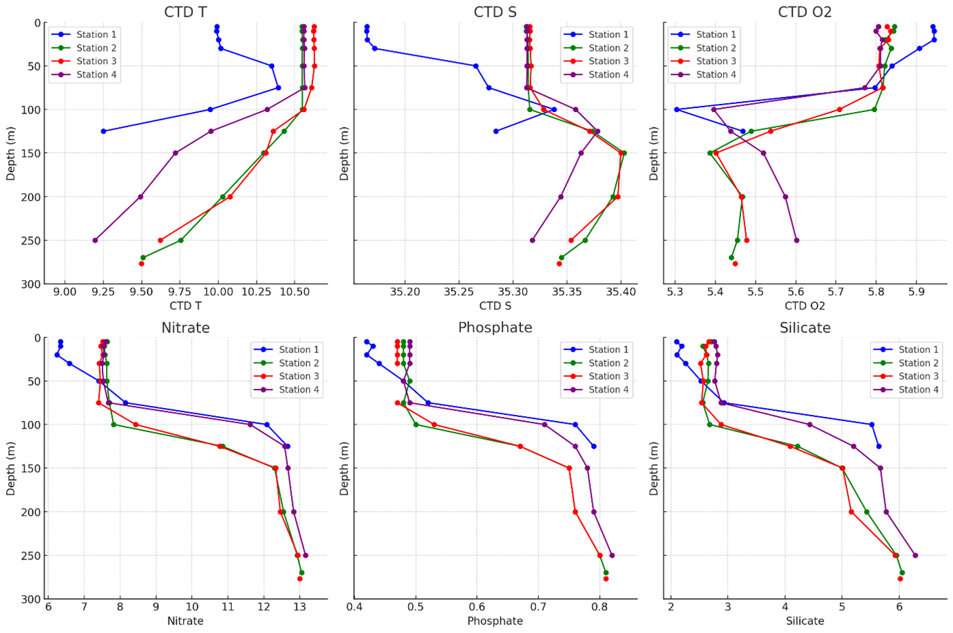
However, to get some data on the wake effects, we planned three cross shelf CTD transect with 12 stations (Figure 5). Each station should include water samples for nutrient, and eDNA analysis as well as WP2 net hauls for looking at plankton community / distribution. Furthermore, we planned to use an MSS Probe, also known as a MICRO-CTD (Figure 4) to study the wake effect in transect going from the safety sone and down shelf (North-East) and from the safety sone and up shelf (South-West) and across the same depth range on the shelf north and south of HT (Figure 5). However bad weather condition allowed us only 23 working hours at HT over the entire cruise, thus we only managed to sample four of the 12 CTD transect stations (Table 1). In addition, we had a CTD station in the circle of the Lander and FAD position (Figure 3).
MICRO-CTD (MSS probe)
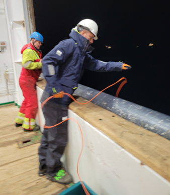
The MSS Probe was deployed from the hangar by hand. During the probe sampling the vessel needs to be drifting. This to avoid current from propeller and trusters, affecting the measurement. We were not allowed to have the vessel drifting within HT or within its 500 m safety zone. Thus, this probe was only used on the stations outside HT safety zone. We conducted two MSS probe stations at HT (St. 1. and St. 3, Figure 5 and Table 1). This work was done on or second trip to HT, on the 25th-26th of October, then we had a 14-hour weather window.
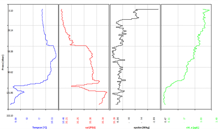
Figure 4. Above left, the MSS probe (MSS90L) also known as MICRO-CTD, right the same probe being deployed by hand from the hangar. Below: Example of the MSS profiles collected at HT St.1. Temperature (blue), salinity (red), epsilon (black) and chlorophyll-a (green) profiles in the layer 0-130m are shown. It is interesting to note a cold and fresh intrusion at ~110m depth with a small dissipation signature. Pictures by A.C. Utne Palm.
Nutrients
We took samples at four stations at HT all on the central cross shelf transect (St.1, St. 2, St.3, and St.4, see Table 1). St. 2 was a central station inside HT (marked by a star in Figure 5). Nutrients were not taken at our first CTD stations in FAD and Lander circle area (st. 540 and 541) as we were not able to locate the chloroform dispenser (we found the dispenser later).
Nutrient samples: were taken following the standard depth used at IMR: 300 (or deepest), 250, 200, 150, 125, 100, 75, 50, 30, 20, 10, 5m depth.
Nutrient Results: from the four stations cross shelf central transect is shown in Figure 6.
Table 1. The activity and sampling at Hywind Tampen during the first day and the last two days. Latitude and longitude data are given in degrees min and sec.
Activity
Comments
St.no.
Micro CTD
RNA
eDNA
Nutients
Plankton
Date
Time (UTC)
WP2
5 nm outside HT
14
controll
20.10.2024
03:29
FAD
FAD out
470
20.10.2024
05:09
Lander
Lander in
471
20.10.2024
07:43
CTD and water
in Lander circle
540
10, 90, 260m
20.10.2024
08:16
WP2
in Lander circle
15
260-0 m
20-0m, 90-0m, 260-0m
20.10.2024
08:41
CTD and water
in Lander circle
541
10, 90, 260m
20.10.2024
09:43
Acoustic transect
with sonar
20.10.2024
10:47 to 12:45
Acoustic transect
without sonar
25.10.2024
09:23 to 10:49
Pelagisk trawle
with DeepVision
502
25.10.2024
11:25
Lander out
Lander out
481
25.10.2024
16:10
CTD and water
CTD transect (st.2)
553
10, 130, 270m
10m, 130, 270m
25.10.2024
16:14
WP2
CTD transect (st.2)
26
150-0m, 250-0m
25.10.2024
17:36
CTD and water
CTD transect (st.2)
554
12 bottl. 270 to 5 m
25.10.2024
18:13:00
CTD and water
CTD transect (st.1)
555
10, 100, 130m
130, 100, 10m
25.10.2024
19:12
WP2
CTD transect (st.1)
27
130-0m, 90-0m, 20-0m
25.10.2024
19:28
CTD and water
CTD transect (st.1)
556
9 bottl. 130 to 5m
25.10.2024
19:59
Micro CTD
CTD transect (st.1)
482
3x 130-0m
25.10.2024
20:13
Acoustic transect
across shelf HT
25.10.2024
21:00 to 00:20
CTD and water
CTD transect (st.3)
557
10, 130, 280m
280, 130, 10m
25.10.2024
21:27
WP2
CTD transect (st.3)
28
250-0m, 130-0m
25.10.2024
21:45
CTD and water
CTD transect (st.3)
558
10, 130, 277 m
12 bottl. 277 to 5 m
25.10.2024
22:18
Micro CTD
CTD transect (st.3)
483
3x 270-0m
25.10.2024
22:36
CTD and water
CTD transect (st.4)
559
10, 100, 330m
12 bottl. 330 to 5m
25.10.2024
23:31
WP2
CTD transect (st.4)
29
300-0m
25.10.2024
23:46
WP2
CTD transect (st.4)
30
130-0m
26.10.2024
00:10
Figure 5. Figure shows the 3 planned cross shelf transect lines –holding 12 stations for MSS probe stations, CTD, nutrients, eDNA and plankton net sampling (WP2 net). Only the four stations marked with blue circles were sampled. At St. 4 and St. 2 we did not sample with the MSS probe. The red box indicates the wind farm area. See Table 1 for data sampled, and Figure 6 for CTD and nutrient results.Figure 6. Results showing the environmental data: temperature (CTD T), salinity (CTD S), oxygen (CTD O2), nitrate, phosphate, silicate, from the CTD transect across shelf at Hywind Tampen. See Figure 5 and Table 1 for station information.
2.1.4. Plankton samples (WP2 and water bottles)
By Allesandro Bergamasco, CNR-ISMAR, Venice, Italy.
To look at the plankton community structure we also conducted net hauls at the stations. Given that the MAMUT Multinet is impossible to use under bad weather conditions, we had to use the WP2.
Besides looking at the community, the copepods sampled in WP2 were used to look at possible changes in RNA due to exposure to noise (see section 2.2.1 below). Our first WP2 station was a plankton haul (St. 14) 5 nm outside HT, this was to get control animals (none exposed copepods) for the RNA study. This first plankton sample was also used as a test sample for practicing handling of plankton samples (following the ISMAR protocol in Appendix 7.3.), that was important as we had six master students onboard as part of the scientific crew. The first WP2 inside HT (st. 15) was used as sample of exposed animals (RNA sample, see section 2.2.1. and Table 4).
A total of five WP2 stations at HT were used for sampling plankton community in addition to four CTD stations with water bottle samples (Table 1).
Zooplankton analyses are currently underway. Concerning the copepod fauna, some first descriptive aspects can be given. Oithonidae and Acartiidae are generally dominant in the community, while Metrinidae family assumed greater importance after the storm (25/26 October). The opposite seems to exhibit Centropagidae specimens whose abundance decreased. Overall, the former (corresponding to Lander station, St.15) was a richer sample than the later one (sample corresponding to CTD 553), both qualitatively and quantitatively. As for Holo-/Meroplankton, Siphonophores were the main component of the community.
Identification of the specimens at the highest taxonomic level is ongoing. Comparison of genetic data (eDNA metabarcoding) referred to plankton taxa will be crucial.
2.1.5 eDNA
By M. Majaneva Norwegian Institute for Nature Research, Trondheim, Norway.
A simple way of sampling what animals are present in an area is by extracting eDNA from water samples. Consequently, we collected water samples for eDNA analysis at all four CTD stations (see Table 1, Figure 5). In addition to the eDNA stations recorded in the log and Table 1, we also collected an eDNA sample from the onboard water system during the transit from HT to Sognefjorden on the afternoon of October 21st.
eDNA sampling: From each station, we sampled 3x 5 litre water from three depths: surface, pycnocline and bottom. Depth of the surface sample was ca. 10 m below surface and bottom sample was ca. 20 m above the bottom. Due to windfarm structure on the bottom we were not allowed to sample closer to the seafloor. Before sampling water, we took a CTD haul to find the pycnocline. In total, we took 36 samples (4 stations, 9 samples). In addition, we took air control samples after samplings and from the fresh water that was used to wash sampling units (4 controls) and some extra surface samples from a hose (3 stations inside Hywind and 3 stations on our way back to Norway). The samples were filtered, using three 500-mL filter holders (Nalge Nunc International Corporation, Rochester, USA) connected to an EZ-Stream peristaltic pump (Merck KGaA, Darmstadt, Germany). The used filters were 2.0 µm glass fiber filters (Merck KGaA). Immediately after filtration, filters were submerged into buffer ATL (Qiagen GmbH, Hilden, Germany) until DNA extraction. Between filtrations, the filtration units were washed with bleach and fresh water. DNA was extracted using the Nucleospin Plant II Midi kit (Macherey-Nagel GmbH, Düren, Germany), and amplified in PCR reactions using fish-specific mitochondrial 12S rRNA gene primers MiFish-U-F and MiFish-U-R (Miya et al. 2015). The amplicons were paired-end sequenced (2x150 bp) using Illumina NovaSeq 6000 machine. Sequence reads were quality filtered using dada2 (Callahan et al. 2016) and taxonomically assigned using blastn (Zhang et al. 2000) against MitoFish (Zhu et al. 2023) nucleotide database.
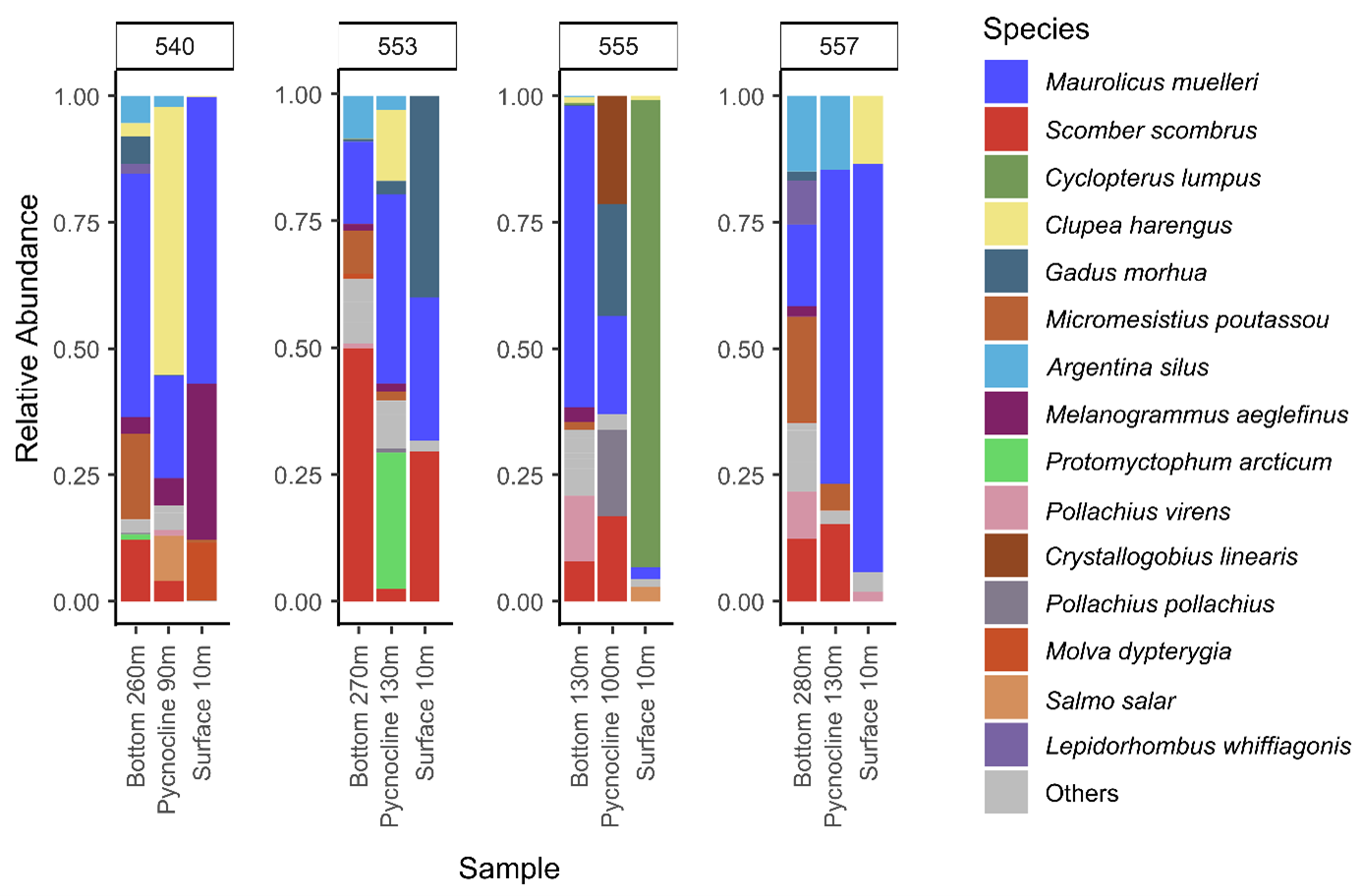
eDNA Results: Most abundant species included, for example, the mesopelagic species silvery lightfish (Maurolicus muelleri), the species that we saw in the DeepVison trawl transect trough the windfarm (Figure 10) mackerel (Scomber scombrus), herring (Clupea harengus) that are typical (meso-)pelagic fish in the area (Figure 7). Blue whiting (Micromesistius poutassou) and many gadoid species i.e. Atlantic cod (Gadus morhua), saith (Pollachius virens). Interestingly lump sucker (Cyclopterus lumpus) DNA was also found. A complete list of fish species is given in Table 2. In addition to fish, there were five species of whales detected with low read abundance: white-beaked dolphin (Lagenorhynchus albirostris) at CTD station 553, Atlantic white-sided dolphin (Lagenorhynchus acutus) at CTD station 557, long-finned pilot whale (Globicephala melas) at CTD station 557, Risso's dolphin (Grampus griseus) at CTD station 557, and harbour porpoise (Phocoena phocoena) at CTD stations 540 and 555.
Figure 7. Relative abundance of 15 most abundant fish species at the 4 stations sampled, based on eDNA in water. At each station, three replicates were sampled at each depth (10m below surface, at pycnocline, and 20m above bottom); these samples were merged for this figure.
Table 2. List of species in the Hywind Tampen according to water eDNA samples. A total of 13 species were removed from this table due to an obvious cross-contamination in our sequencing run. The removed species are either freshwater species or coastal species that were very abundant in samples that were sequenced together with th Hywind Tampen samples. If a species is present in a sample, there is several hundreds or thousands of reads. These contaminants had less than 20 reads in the samples. So it is statistically safe to remove them.
Class
Order
Family
Genus
Species
Actinopteri
Argentiniformes
Argentinidae
Argentina
Argentina silus
Actinopteri
Argentiniformes
Microstomatidae
Nansenia
Nansenia sp. 1
Actinopteri
Caproiformes
Caproidae
Capros
Capros aper
Actinopteri
Carangiformes
Carangidae
Trachurus
Trachurus trachurus
Actinopteri
Clupeiformes
Clupeidae
Clupea
Clupea harengus
Actinopteri
Clupeiformes
Clupeidae
Sprattus
Sprattus sprattus
Actinopteri
Gadiformes
Gadidae
Boreogadus
Boreogadus saida
Actinopteri
Gadiformes
Gadidae
Gadiculus
Gadiculus argenteus thori
Actinopteri
Gadiformes
Gadidae
Gadus
Gadus morhua
Actinopteri
Gadiformes
Gadidae
Melanogrammus
Melanogrammus aeglefinus
Actinopteri
Gadiformes
Gadidae
Micromesistius
Micromesistius poutassou
Actinopteri
Gadiformes
Gadidae
Pollachius
Pollachius pollachius
Actinopteri
Gadiformes
Gadidae
Pollachius
Pollachius virens
Actinopteri
Gadiformes
Gadidae
Trisopterus
Trisopterus esmarkii
Actinopteri
Gadiformes
Gadidae
Trisopterus
Trisopterus minutus
Actinopteri
Gadiformes
Lotidae
Brosme
Brosme brosme
Actinopteri
Gadiformes
Lotidae
Molva
Molva dypterygia
Actinopteri
Gadiformes
Lotidae
Molva
Molva molva
Actinopteri
Gadiformes
Macrouridae
Coryphaenoides
Coryphaenoides rupestris
Actinopteri
Gadiformes
Merlucciidae
Merluccius
Merluccius merluccius
Actinopteri
Gadiformes
Phycidae
Phycis
Phycis blennoides
Actinopteri
Gobiiformes
Gobiidae
Crystallogobius
Crystallogobius linearis
Actinopteri
Gobiiformes
Gobiidae
Pomatoschistus
Pomatoschistus minutus
Actinopteri
Lophiiformes
Lophiidae
Lophius
Lophius piscatorius
Actinopteri
Myctophiformes
Myctophidae
Benthosema
Benthosema glaciale
Actinopteri
Myctophiformes
Myctophidae
Notoscopelus
Notoscopelus elongatus kroyeri
Actinopteri
Myctophiformes
Myctophidae
Protomyctophum
Protomyctophum arcticum
Actinopteri
Ophidiiformes
Carapidae
Echiodon
Echiodon drummondii
Actinopteri
Osmeriformes
Salangidae
Mallotus
Mallotus villosus
Actinopteri
Perciformes
Anarhichadidae
Anarhichas
Anarhichas sp. 1
Actinopteri
Perciformes
Cyclopteridae
Cyclopterus
Cyclopterus lumpus
Actinopteri
Perciformes
Sebastidae
Helicolenus
Helicolenus sp. 1
Actinopteri
Perciformes
Sebastidae
Sebastes
Sebastes sp. 1
Actinopteri
Perciformes
Triglidae
Triglidae sp. 1
Actinopteri
Pleuronectiformes
Pleuronectidae
Glyptocephalus
Glyptocephalus cynoglossus
Actinopteri
Pleuronectiformes
Pleuronectidae
Hippoglossoides
Hippoglossoides platessoides
Actinopteri
Pleuronectiformes
Pleuronectidae
Microstomus
Microstomus kitt
Actinopteri
Pleuronectiformes
Scophthalmidae
Lepidorhombus
Lepidorhombus whiffiagonis
Actinopteri
Salmoniformes
Salmonidae
Oncorhynchus
Oncorhynchus mykiss
Actinopteri
Salmoniformes
Salmonidae
Salmo
Salmo salar
Actinopteri
Scombriformes
Scombridae
Scomber
Scomber scombrus
Actinopteri
Scombriformes
Scombridae
Thunnus
Thunnus sp. 1
Actinopteri
Stomiiformes
Sternoptychidae
Maurolicus
Maurolicus muelleri
Actinopteri
Syngnathiformes
Callionymidae
Callionymus
Callionymus maculatus
Actinopteri
Uranoscopiformes
Ammodytidae
Ammodytidae sp. 1
Chondrichthyes
Chimaeriformes
Chimaeridae
Chimaera
Chimaera monstrosa
2.1.5. Acoustic study – and trawling with DeepVision
Hywind Tampen might attract fish do to all the added structure or it might scare fish away by noise and activity. We therefor want to look at any possible attraction or avoidance effect by conducting an acoustic transect from within Hywind Tampen to 5 nm from the farm (Figure 8). To ground truth what we saw on the acoustics we used an open-ended pelagic trawl with a camera unit called DeepVision, that takes pictures of the catch as it passes through the trawl (Figure 9).
With a limited number of hours available for work at HT, we decided to focus on the transect through HT (Figure 8). Of these we had three: i) with echosounder and sonar on, ii) with echosounder and without sonar and iii) with echosounder and with open pelagic trawl and DeepVision (Table 1). In addition, we have acoustical data from our entire period at HT. This includes a cross shelf transect conducted during the CTD transect St. 1 to St. 4 (on the 25th -26th of October).
Figure 8. Drawing shows the transect conducted by G.O. Sars trough the Hywind Tampen (dotted blue line). It starts and ends 3 nm (5.5 km) from the safety zone (yellow line). Dotted circle between HY07 and HY08 (turbine 7 and 8) is the Lander site shown in Figure 3. Suction anchors are marked SA- and turbines HY-number. Brown full and - dotted lines are cables.
Transect through Hywind Tampen
The first acoustic transect was conducted on the 20th of October between 12:45-14:45. It started 3nm from the safety zone and went from south to north in the centre between the two rows of the five and the six turbines. We used sonar (MS70 multibeam sonar) hoping to detect fish to the side of the vessels transect.
Second transect was on the 25th of October between 12:25 and 12:49. Entering from north 3nm from safety zone. This time we only used the RV G.O. Sars multi-beam echosounders and not the sonar, we went against the wind. Only nine of the eleven turbines were running (HY04 and HY02 was not running).
The third transect was with a pelagic trawl (Harstad trawl), on the 25th of October ~13:00 and 16:00, going from 3nm south of safety zone trawling with the wind northwards. Shooting at 13:05. It was at 175-185 m depth (13:25) at ~1.5 nm from the safety zone. In the centre of the park the trawl was at ca 120 m. At 14:20 between HY07-HY08 and outside HY05 the trawl was at 180-200 m. The trawl was at 150 m depth last part inside and outside of the park. The trawl was at surface when ~1 nm outside safety zone North of the park (15:54).
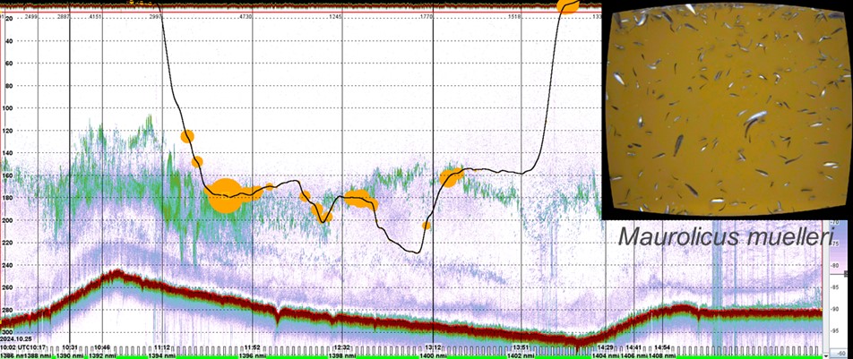
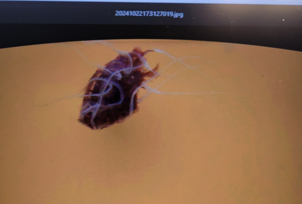
DeepVison results: The dominant species seen on DeepVision in the acoustic Sound Scattering Layers were dominated by the mesopelagic fish Maurulicus muelleri (Figure 10), some krill (Figure 12) and gelatinous zooplankton, among which the siphanopora Siphonophorer Apolema sp. (Norwegian name: Perlemors manet) was observed several times (see Figure 11).
When trawling the vessel speed was ≥3 nm/h. We caped the trawl >50 m above the bottom, and at a distance of >200 m from the suction anchors.
When trawling the vessel speed was ≥3 nm/h. We caped the trawl >50 m above the bottom, and at a distance of >200 m from the suction anchors.
Figure 9. Deep vision is an open trawl where the catch goes through a camera tunnel before it goes through the open cod end of the trawl. It is used in research to document what is in the different acoustic layers without having to catch the fish. It is developed by Scantrol in collaboration with IMR. Picture by K. de Jong.
Figure 10. Showing the DeepVision results being displayed in LSSS, from the DeepVison trawl transect inside the windfarm. The black line shows where the trawl is. Yellow circles shows where the catches are large or when large numbers of organisms pass through DeepVison (bigger circle bigger catch/ more individuals). The typical camera view from the yellow circles in this trawl station is shown in upper right corner, dominated by the mesopelagic fish Maurolicus muelleri.
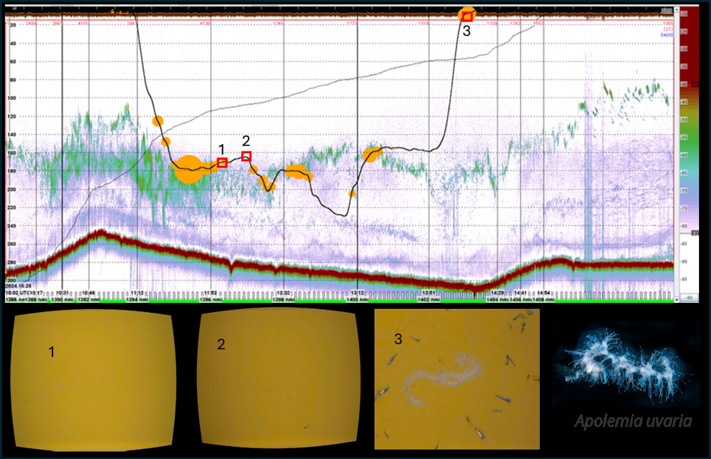
Figure 11. Showing the DeepVision results being displayed in LSSS, from the DeepVison trawl transect inside the windfarm. The black line shows where the trawl is. The red squares shows when during the trawl track the Siphonophorer Apolema sp. (Norwegian name: Perlemors manet) was observed in DeepVision.
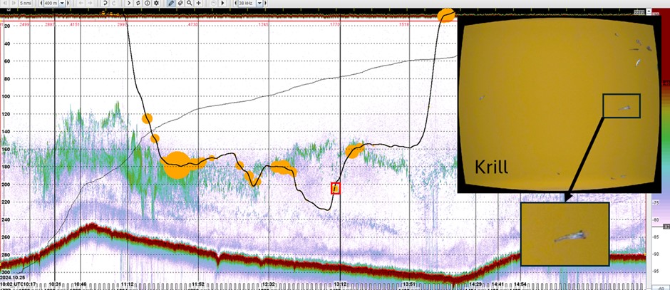
Figure 12. Showing the DeepVision results displayed in LSSS, from the DeepVison trawl transect inside the windfarm. The black line shows where the trawl is. The red squares shows when during the trawl track we observed most krill.
2.1.6. Bird surveys at Hywind Tampen
By E.J. Critchley, Norwegian Institute for Nature Research, Trondheim, Norway.
Bird surveys were carried out at all opportunities both inside and outside the wind farm by two bird observers on deck. Each time a bird was detected the following data fields were recorded:
Time
Species (or group e.g. gull)
Size (estimate if it was small, medium or large)
Large = e.g. Great black-backed gull
Medium = e.g. Fulmar
Small = e.g. Finch
Number of birds – in some case large flocks were observed
Distance from the boat (in metres)
Behaviour
Transiting – flying in a straight path
Searching – circling behaviour but not actively foraging
Foraging
Sitting on the water
Following the boat
Turbine influence – noted if the bird was flying close to the turbine
Flight direction
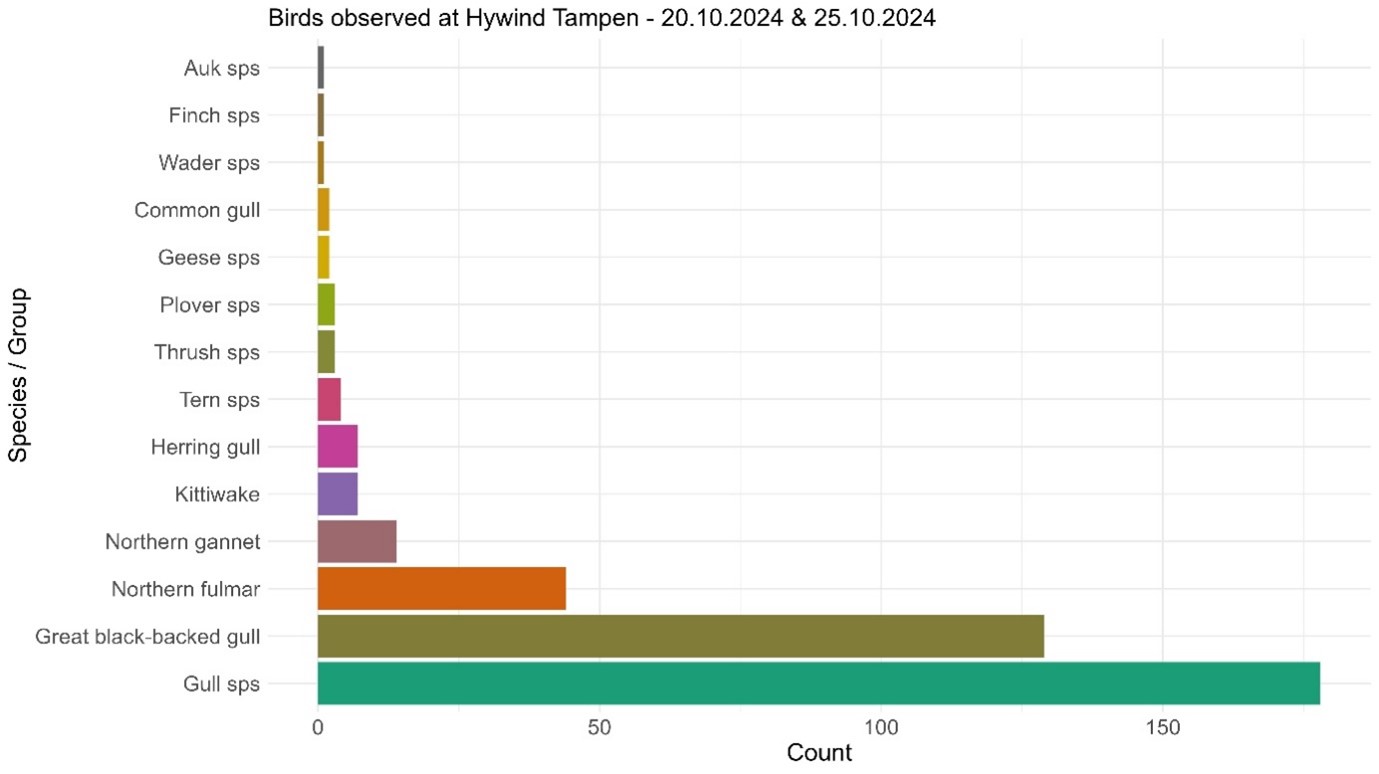
Bird survey results: In total 163 birds were observed, with the most common being unidentified gull species and Great black-backed gulls. Approximately 4% of the birds observed were presumed to be migrating birds, e.g. tern, thrush, plover, geese, wader and finch species. The largest number of birds were seen on the afternoon of October 25th, corresponding with the deployment of the Deep vision trawl and the third acoustic transect. Large numbers of gulls and fulmars were attracted to the vessel.
Figure 13. Showing counts of different species groups of birds at Hywind Tampen during daylight hours on the 20th and the 25th of October 2024.
2.2. Activity in Sognefjorden (21st to 25th of October)
We arrived in Sognefjorden around 22:30 21st of October – and left on the 25th at ~01:45.
During our time in Sognefjorden we conducted 10 CTD standard stations (with nutrients). These were station: S02 to S11. These are all listed in the log and will not be mentioned any further in this cruise report, as they were not part of this planed cruise, but valuable data for IMR salmon lice model.
2.2.1. Behavioral observation on Calanus spp. Swimming behavior exposed to ship noise
By F. Viotti and S. Kühn, Coastal Ecology, Research and Technology Centre West Coast, Kiel University, Büsum, Germany.
This experiment was initially planned to take place around the Hywind Tampen wind farm to investigate the effects of continuous low-frequency underwater noise on copepod swimming behavior. However, since these experiments required calm weather conditions—which were not met—we implemented a Plan B experiment to study the effects of underwater ship noise on copepod swimming behavior instead. In this experiment, copepod behavior was monitored during an intermittent exposure period, where they were exposed to approaching - passing ship noise, and compared to a negative control, in which the research vessel remained near the experimental setup (continuous exposure).
In addition to the experiments on copepod swimming behavior, we collected RNA samples under different environmental conditions to investigate potential transcriptional responses of copepods to low-frequency noise.
In-situ studies on the effects of anthropogenic noise on copepods are rare but crucial for understanding how increasing underwater noise pollution impacts marine ecosystems. By conducting field-based experiments, we can gain more ecologically relevant insights into copepod responses compared to laboratory conditions, ultimately improving our understanding of potential disruptions to marine food webs.
Methods
Experimental Animals
Animals were caught the days before the cruise at the IMR Research Station, in Austevoll, using light traps (Kühn et al., 2022) at 3-5 m depth, and during the cruise using WP2 nets from 100 - 0 m.
Cage set-up
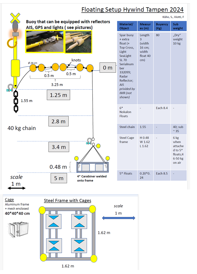
The cage consists of four replicate plankton mesh cages, holding two go-pro cameras for 3D observation of behaviour, and a hydrophone. All four cages are placed in a common steel frame. This frame is caped at a depth of 5 m by rope and buoys. A 3,25 m chain of buoys (sjøhund) was added to the rope to damper the wave action. To track the position of the cage an AIS was added to the top of its surface buoy (Figure 14).
We always consider surface current direction before dropping off by the vessels winch. The cage setup was retrieved by the “sjøhund” (chain of buoys at the surface) and lifted by winch at G.O. Sars. Experimental Setup.
Figure 14. Detailed information of the Cage set-up, used for in-siu study of zooplankton behaviour related to sound. The set-up is designed by Saskia Kühn and Fabio Viotti.
Cage design: Four cages (40 × 40 × 40 cm) with an aluminum frame enclosed by 100 µm mesh, (Figure 14). Three of the cages each contained a transparent observation chamber (10x10x18 cm3), with two GoPro cameras (model Hero 8) mounted at a 90° angle to capture 3D trajectories of the copepods. In two of these cages, video recordings were conducted under white light conditions, while the third was recorded under infrared (IR) light.
The fourth cage was designated for RNA sampling and contained six small plastic containers (110 mL) with open lids enclosed by 100 µm mesh to allow water exchange while keeping the samples contained.
Experiment procedures
All six cage experiments had the following start position: start ca N 61° 07,291 – E 6° 32,203 (degrees min, sec).
Passage exposure:
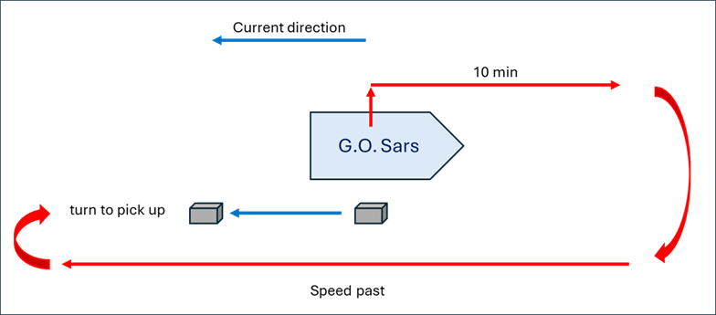
G.O. Sars moves slowly away from the cage (current pulls the cage away from the vessel). Vessel engine going slow, trusters are off. When the vessel is at ca 1000 m distance to the cage, the vessel, turned the engine on full power (full speed) running towards the cage and passing it at 100 m distance. Whereafter the vessel turned and picked up the cage (total time in water ca 40 min) (Figure 15).
Figure 15. Fast passing from 1000 m to 100 m distance.
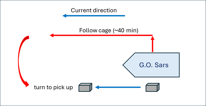
Control – negative control:
Continues noise experiment. G.O. Sars uses full speed on trusters follow the cage at a distance of 25-100 m for 40 min (Figure 16).
Figure 16. Negative control research vessel keeps close and make continuous noise.
An overview of the date and time of each trial is given in Table 3, and a more details description of each trail follows below.
Table 3. Overview of the date and time of each trial. For more details see text below.
Date
Exp. #
Trial
Time In
Time Out
Individuals
22.10.2024
1
Exposure
09:02
09:48
30 (video) + 30 (RNA)
22.10.2024
2
Neg. Control
17:20
18:05
30 (video) + 30 (RNA)
23.10.2024
3
Neg. Control
10:09
11:00
30 (video) + 30 (RNA)
23.10.2024
4
Exposure
16:01
16:46
30 (video) + 30 (RNA)
24.10.2024
5
Exposure
09:06
09:44
30 (video) + 30 (RNA)
24.10.2024
6
Neg. Control
16:02
16:59
30 (video) + 30 (RNA)
Description of each trail
Exp. 1. Passing exp. (st. 472) on the 22.10.24 at 09:02-09:48. G.O. Sars Slowly moved from the cage slowly, helped by the current and carefully trusting away to ca 200 m distance. Whereafter turned off truster and runed engine slowly. Then after 1000 m (09:16) turned vessel, turned engine power full speed passing by the cage at 100 m distance (09:22). Turned and picked up the cage ca 09:42 (total time in water ca 40 min).
Exp. 2. Follow - negative control (st. 473) on the 22.10.24 at 17:20-18:05. A Catamaran passenger boat passed us just after the cage entered the water. Distance between G.O. Sars and cage ca 50 -150 m for 40 min. G.O. Sars used full speed on trusters to make maximum noise.
Exp. 3. Follow - negative control (st. 475) on the 23.10.24 at 10:09-11:00. G.O. Sars truster away from the cage and stayed at 25-65 m distance for 40 min, with trusters on full speed.
Exp. 4. Passing exp. (st. 477) on the 23.10.24 at 16:01-16:46. G.O. Sars moved away slowly using trusters and current drifting until 100m distance Turn on engine and drove off (3-4 knots) to 1000 m (16:18) turns, passes (16:25) at 145 m. Finished at 16:40.
Exp. 5. Passing exp. (st. 479) on the 24.10.24 at 09:06-09:44. G.O. Sars trusting and drifting slowly away to 100m (09:12) speed 4,5 knots (asked for 3-4 knots) to 1000 m distance (09:21). Passed at (09:26) at 100 m distance 10.8 knot. Out of water at 09:44.
Exp. 6. Follow – negative control (station number missing) on the 24.10.24 at 16:02-16:59. Follow with full speed on trusters at 50-100 m distance for ca 50 min.
Sound recordings
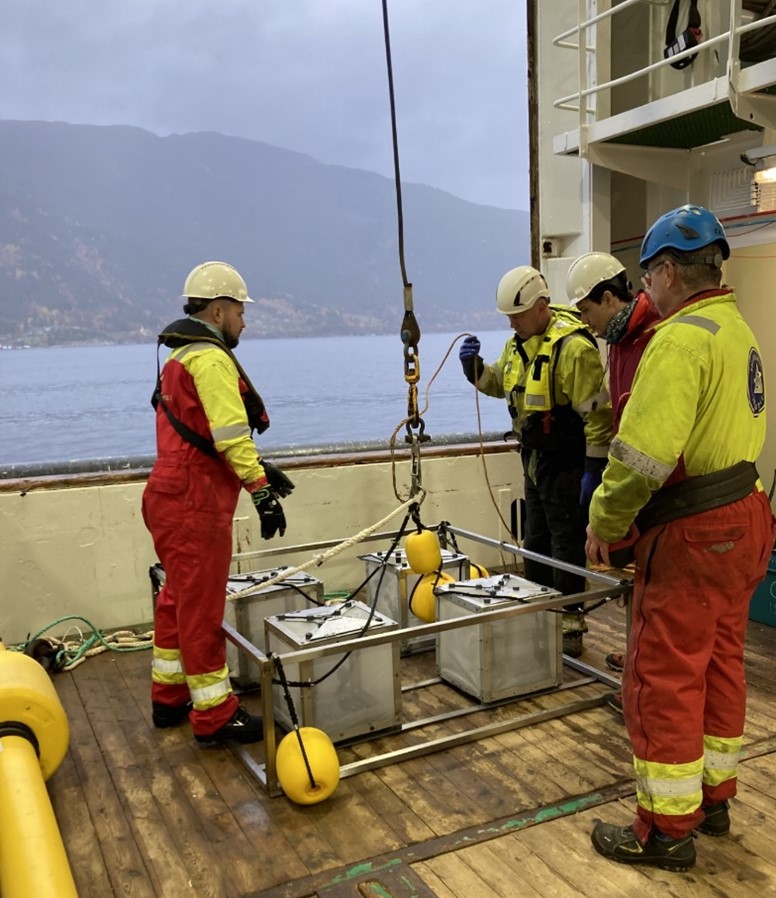
A SoundTrap HF 300 (sensitivity of -176.3 dB) was placed in one of the cages of the experimental floating setup for later sound – video synchronization to correlate sound levels to potential behavioral changes (Figure 17).
Figure 17. Cage setup: getting ready to be deployed (top), being deployed (midle), and starting the experiment by synchronising camera and hydrophone recordings (below). Pictures by A.C. Utne Palm.
Data and samples
Sound: In total we collected 287 minutes of underwater recordings of which 155 were made during the negative control trials and 132 were made during the exposure trials. The sound levels recorded reached a maximum of 150.34 dB (recorded during the negative control on the 22.10.2024) and a minimum of 75.78 dB (recorded during the exposure trial on the 22.10.2024).
Videos: In total we collected 1722 minutes of video recordings of which 930 were made during the negative control trials and 792 were made during the exposure trials.
Animals: A total of 180 animals (90 animals during exposure, and 90 animals during negative control) were recorded. The copepods were preserved in 2.5 % formaldehyde et the end of the experiment.
RNA samples
During the experimental period, we collected a total of 25 RNA samples, each containing 10 to 14 Calanus spp. a total of 356 copepods. One sample was taken outside Hywind Tampen, and another inside, using WP2 nets. Additionally, we collected 9 samples from the experimental and the control groups. To account for potential handling stress, we included three additional control samples. Furthermore, we collected two “blank” controls, where copepods were taken directly from Sognefjord without any controlled exposure (Table 4).
RNA preparation: Copepods were preserved in 1 to 1.5 mL RNA-Protect in a fridge until being shipped to the consortium partners at the University of Padua for RNA analysis led by Alessandro Vezzi.
Table 4. RNA overview. This table shows the Date of fixation – Copepod genus – Catching Site and Date – The number of copepods per sample – Experimental condition.
Sample
Date
Genus
Caught
DateCatch
# cop
Experimental Condition
1
20.10.2024
Calanus sp.
outside Hywind Tampen
20.10.2024
14
Windpark Control
2
20.10.2024
Calanus sp.
Hywind Tampen
20.10.2024
12
Windpark Exposure
3
22.10.2024
Calanus sp.
Austevoll
16.-17.10.2024
10
Passage Exposure
4
22.10.2024
Calanus sp.
Austevoll
16.-17.10.2024
10
Passage Exposure
5
22.10.2024
Calanus sp.
Austevoll
16.-17.10.2024
10
Passage Exposure
6
22.10.2024
Calanus sp.
Austevoll
16.-17.10.2024
10
Negative Control
7
22.10.2024
Calanus sp.
Austevoll
16.-17.10.2024
10
Negative Control
8
22.10.2024
Calanus sp.
Austevoll
16.-17.10.2024
10
Negative Control
9
22.10.2024
Calanus sp.
Sognefjord
22.10.2024
10
Negative Control
10
23.10.2024
Calanus sp.
Austevoll
16.-17.2024
10
Negative Control
11
23.10.2024
Calanus sp.
Sognefjord
23.10.2024
10
Negative Control
12
23.10.2024
Calanus sp.
Austevoll
16.-17.2024
10
Negative Control
13
23.10.2024
Calanus sp.
Austevoll
16.-17.2025
10
Passage Exposure
14
23.10.2024
Calanus sp.
Austevoll
16.-17.2026
10
Passage Exposure
15
23.10.2024
Calanus sp.
Austevoll
16.-17.2027
10
Passage Exposure
16
24.10.2024
Calanus sp.
Sognefjord
24.10.2024
10
Passage Exposure
17
24.10.2024
Calanus sp.
Sognefjord
24.10.2024
10
Passage Exposure
18
24.10.2024
Calanus sp.
Sognefjord
24.10.2024
10
Passage Exposure
19
24.10.2024
Calanus sp.
Sognefjord
24.10.2024
10
Negative Control
20
24.10.2024
Calanus sp.
Sognefjord
24.10.2024
10
Negative Control
21
24.10.2024
Calanus sp.
Sognefjord
24.10.2024
10
HandlingControl
22
24.10.2024
Calanus sp.
Sognefjord
24.10.2024
10
HandlingControl
23
24.10.2024
Calanus sp.
Sognefjord
24.10.2024
10
HandlingControl
24
24.10.2024
Calanus sp.
Sognefjord
24.10.2024
10
"Blank" Control
25
24.10.2024
Calanus sp.
Sognefjord
24.10.2024
10
"Blank" Control
2.2.2. Trawling with DeepVision
We conducted three trawls hauls with DeepVision inside Sognefjorden. This was to test out that everything worked ok, and to get the team familiar with the equipment and handling of data. Also, we wanted to see if we could fine the deep-water jelly Periphylla periphylla, and get some ide of its abundance, size – and depth distribution. Thus, we made one trawl (DeepVision St. 499) after dusk (19:00-21:50). Total time trawling 1 h 42 min. Trawling ~20 min per depth: 400 m, 230m, 50m. We registered Periphylla periphylla at all depth (Figure 18). And one (DeepVision St. 500) during daytime (12:45 – 14:33). Trawling ~15 min per depth: 400m, 200m and 60m.
Figure 18. Shows the deep-sea jelly Periphylla periphylla in DeepVision (st 499), in Sognefjorden.
2.2.3. Acoustic communication experiments by Develogic
Develogic conducted several (St. 474, St. 478 and one without station number) signal tests experiments for communication at different depths: 300m, 500m and 1050 m. The later the deepest possible location in Sognefjorden. The test consists of two devices: one deployed on the CTD wire and the second lowered in water from overboard.
Each single test communication session took around 2 hours. During the communication session 20-30 min the vessel thrusters had to be switched off (incl. DP system), to avoid interfering with the acoustic communication channel.
2.3. Priorities taken as weather conditions restricted our work time
Due to bad weather condition, leaving us only 23 hours available for work at Hywind Tampen, we had to pick the most important tasks. After priority 1. FAD and Lander was dealt with, we decided to take a CTD (st. 540 and 541) and WP2 (st. 15) stations within close distance to the Lander and FAD (orange circle, Figure 3). After that we took the central CTD station on the acoustic transect through HT (marked with a star in Figure 5). At this station we conducted two CTD stations (St. 553 and 554) and one WP2 station (St.26), see Table 1. To save time we used this star station as the central station St. 2 in our following task, the transect across the HT shelf (Figure 5). In the cross shelf transect we conducted St. 1, the shallowest station, skipped the next station on the transect, which was replaced by the star station (St. 2) and continued with St. 3 and St. 4. We managed the full transect concerning CTD, nutrients, eDNA and plankton data, but had to skip the MSS probe sample on the last station (St. 4), as the wind was picking up again. Leaving us with data from only two MSS probe stations (St. 1 and St. 3), as we were not allowed to use the MSS probe inside the park (on St. 2) (see Table 1).
Regarding the acoustic transects with and without DeepVision, we decided to focus on conducting three replicate transects through HT (ca 5 hours), as the flower transect around HT would take more time than we had available (15-20 hours). Instead, we collected acoustic data along the CTD-transect perpendicular to the transect through the wind farm.
3-Samples and data handling
All plankton samples taken on this cruise was conducted under guidance by researchers from ISMAR, Italia, and brought back to be analysed at their lab, as part of the Orchestra project.
Experimental data on Calanus spp. were conducted by and analysed by researchers from University of Kiel, as part of the Orchestra project.
RNA later samples were handled on board by the researchers from Kiel University and was later shipped on to University of Padova for analysis, as part of the Orchestra project.
eDNA samples taken at this cruise was conducted under guidance of NINA, Norway, and brought back to be analysed at their lab., as part of the WindSys project.
Nutrient samples were analysed at IMR, as part WindSys and Orchestra.
DeepVision data, is analysed by IMR, as part WindSys.
Acoustic data is scrutinised by IMR, as part WindSys.
Lander data is part of WindSys and will be analysed by different partners. Hydrophone data will, after cleaned by FFI, be used in a PhD thesis at Geophysical institute, UiB. Acoustical data will be analysed by IMR and as used for master thesis. ADCP data will be analysed by WindSys and Orchestra partners.
Bird data was analysed by NINA.
4-Acknowledgement
We want to thank the kind, professional and efficient crew both on deck and at the bridge of RV G.O. Sars for all their help and extra effort. Complemented by superb food and service from the rest of the G.O. Sars crew. In addition, we were lucky to have six super engaged master students (Thale Styrmoe Hansen, Mathea Aakerøy Jordbru, Lotta Baalerud, Frida Stokkenes Eliasen, Regine Asbjørnsen, Mathea Oceana Sylte Brunvoll) helping us researcher with sampling and experiments conducted onboard. Thanks to the great effort from all participants, we managed to get quite a lot of data from Hywind Tampen and in Sognefjorden. Further we would like to thank the two instrument technicians from Develogic, who came along to help us download data and check the lander before being deployed again. Without support from Equinor we would not have been able to conduct any type of studies at Hywind Tampen. We are very thankful for this opportunity that they have given us and for their conscious and careful planning to ensure our safety when at Hywind Tampen.
5-References
Callahan BJ, McMurdie PJ, Rosen MJ, Han AW, Johnson AJA and SP Holmes, 2016. DADA2: High-resolution sample inference from Illumina amplicon data. Nature Methods 13: 581.
Kühn S, Utne-Palm AC, de Jong K, 2022. Two of the most common crustacean zooplankton Meganyctiphanes norvegica and Calanus spp. produce sounds within the hearing range of their fish predators. Bioacoustics 32(9):1-17. DOI: 10.1080/09524622.2022.2070542
Miya M, Sato Y, Fukunaga T, Sado T, Poulsen JY, Sato K, Minamoto T, Yamamoto S, Yamanaka H, Araki H, et al., 2015. MiFish, a set of universal PCR primers for metabarcoding environmental DNA from fishes: detection of more than 230 subtropical marine species. R Soc Open Sci 2:150088.
Utne-Palm AC, Søiland H, Sveistrup AK, Renner A, Ross R, Moy F, Bakhoday Paskyabi M, Totland A, Hannaas S, de Jong K, Gonzalez-Mirelis G, Hovland T, Pedersen P, Wilhelmsen JF, Majaneva MA, Heum SW, Skjold W, Vågenes S, Skaret G, Corus F, Voronkov A, Vågenes P, Kielland L. Cruise report Hywind tampen 13 to 28 March 2023. Toktrapport No. 10, 2023. https://www.hi.no/hi/nettrapporter/toktrapport-en-2023-10
Zhang, Z., S. Schwartz, L. Wagner & W. Miller, 2000. A greedy algorithm for aligning DNA sequences. Journal of Computational Biology 7: 203–214.
Zhu T, Sato Y, Sado T, Miya M, and Iwasaki W. 2023. MitoFish, MitoAnnotator, and MiFish Pipeline: Updates in ten years. Mol Biol Evol, 40:msad035.
6-Abbreviation and word explanation
ADCP: is an Acoustic Doppler Current Profiler. It is a hydroacoustic current meter similar to a sonar, used to measure water current velocities over a depth range using the Doppler effect of sound waves scattered back from particles within the water column.
Acoustic releaser: is for the deployment and subsequent recovery of instrumentation from the sea floor, in which the recovery is triggered remotely by an acoustic command signal.
CTD: is an oceanography instrument used to measure the electrical conductivity, temperature, and pressure of seawater. Conductivity is used to determine salinity and depth is calculated from pressure.
eDNA or Environmental DNA is DNA that is collected from a variety of environmental samples such as soil, seawater, snow or air, rather than directly sampled from an individual organism. As various organisms interact with the environment, DNA is expelled and accumulates in their surroundings.
Hydrophone: is a microphone designed to be used underwater for recording or listening to underwater sound. Most hydrophones are based on a piezoelectric transducer that generates an electric potential when subjected to a pressure change, such as a sound wave.
LSSS: Large Scale Survey System (LSSS) (pronounced "L-triple-S"). A software product for the interpretation of data from multi-frequency echo sounders. For more details see: https://www.kongsberg.com/maritime/products/oceanscience/
Multi-frequency echosounder: Recent research has shown that simultaneous use of several discrete echo sounder frequencies (multifrequency) not only improves fish stock estimates but can also be used to identify species. This is because each specie has a unique acoustic frequency response. This new and growing understanding greatly improves the value of hydroacoustics to obtain information about marine resources. For more information see: https://www.kongsberg.com/maritime/support/themes/simrad-content-s/scientific-applications/multifrequency-echosounder-operation/
DeepVision: is a camera system that is mounted at the cod-end entrance of the trawl. Here it takes pictures of the catch as it passes through the trawl. It is used to sample fish without having to land or injure the fish, as the fish passes through the open trawl cod-end. For more details see: https://www.deepvision.no/deep-vision-for-marine-research
7-Appendix
7.1. Cruise Timeline
The station numbers in the cruise logbook are given in parentheses.
19th of October
Research crew and equipment on board from 08:00 - leaving Bergen at 17:40
20th of October
Arriving Hywind Tampen area at 05:30
WP2 (st. 14) at 5 nm east of Hywind Tampen. A control station for RNA and test to learn zooplankton sampling procedures.
Before entering Hywind Tampen we called Equinor to open licences (i) allowing us to deploy FAD and Lander, and (iv)deployment and recovery of light weight equipment.
(i). Launch and recovery of Lander and FAD. Operation licence no.: HYT-0002577682
(ii). Acoustic survey with pelagic trawl. Operation licence no.: HYT-0002577706
(iii). Drifting buoy with plankton cage. Operation licence no.: HYT-0002577723
(iv). Deployment and recovery of light weight equipment from main vessel. Operation licence no.: HYT-0002577727.
Deploying Fish Aggregation Devise (FAD)
FAD deployed (st. 470) between 7:00-8:00 (position N61° 18,685, E002° 15, 576 – in degrees min and sec).
Retrieve of Lander
Lander (st. 471) was released at 08:40 on board ca 09:20.
Sampling inside the Lander and FAD circle, No nutrients samples.
CTD eDNA (st. 540) at ca 10:30. Water bottles from: 10 m, 90 m, 260 m eDNA. Inside the Lander and FAD circle.
WP2 (st. 15) at 10:40. Three hauls 20-0m, 90-0m, 260-0m for preserved zooplankton and one 260-0m used for RNA later, exposed.
Captain on phone with Equinor (at 11:00) to inform about activity - opened working licence (ii) Acoustics and trawling through. Turned temporarily off working licence (i) and (vi).
CTD plankton (st. 541) between 11:45-12:00. Water bottles from: 10 m, 90 m og 260 m for preserved zooplankton.
Acoustic transects through Hywind Tampen
No. 1 Acoustic transect through HT with sonar – we observed some echoes.
Left HT at 14:15 – due to bad weather – went to Sognefjorden.
We took one eDNA sample from the water house on deck during the steaming from HT to Sognefjorden.
Arrive in Sognefjorden around 22:30.
21st of October in Sognefjorden
Divelogic (no station number) testing acoustic communication at 600 m and 300 m, ca 10:00 – 12:00.
12:30 -13:30 meeting with scientific presentations from scientists and students.
13:30-16:30 Organised transport of MSS probe from Bergen to Balestrand (probe was delayed and missed the cruise from Bergen). Moboat picked up the Probe in Vangsnes ca 19:30.
16:00 Got in contact with Lars Asplin, IMR, to check if we could help with some CTD stations when in Sognefjorden. Decided to help with CTD and nutrient data from 10 CTD stations in Sognefjorden.
CTD S08 (st. 542) 16:30 the first of the sampled station in Sognefjorden (for Lars Asplin, IMR).
18:30 Meeting to go through Cage exp. Captain, cruise leader, trawl-bas, man on deck, researchers responsible for the experiment.
CTD (st. 543-547) equivalent to station S11, S10, S09, S07, S06. Between 21:00-05:30 (local time). Steam back to station outside Vangsnes for plankton cage exp. after sunrise.
22nd of October in Sognefjorden
St. 1. Cage fast passing exp (st. 472) cage out at 09:02. Vessel slowly moving away from cage, turn at 1000 m distance and come back passing by at 100 m distance full speed. Total time in water ca 40 min.
Testing MSS probe (no station noted). From hangar – vessel drifting. The MSS did not work when entering water – tested several times, stopped working when in water.
WP2 (st. 16 and 17) to 50 m and to 100 m time ca 16:00. To catch experimental animals for Cage exp.
St. 2. Cage follow negative control (st. 473) cage out between 17:20-18:02. Distance between G.O. Sars and cage ca 50-150 m for 40 min. G.O. Sars use trusters to make maximum noise.
DeepVision (st. 499). Between 19:00-21:50. Trawled for ca 20 min per depth: 400 m, 230m, 50m), we observed the jelly, Periphylla periphylla in the trawl.
Steaming to the continue with CTD station during night shifts - 3 h steaming.
23rd of October in Sognefjorden.
CTD stations (st. 548-549) S04, S05. Between 00:40-02:45.
WP2 (st. 18) at 07:00. Depth 50-0m, 150-0m. To catch experimental animals for Cage exp.
Develogic (st 474) at 08:00-09:30. Develogic testing acoustic transport of data – moved to the deepest part of the fjord responder at 1050 m depth.
St. 3. Cage follow negative control (st. 475) cage out between 10:11-11:03. G.O. Sars uses trusters and keep a distance of 25-65 m to the cage for 40 min.
WP2 (st. 19) From 11:10 – 12:10. Three hauls 150-0m. Collection of exp. animals
Testing MSS probe from hangar. 12:20-12:30 did not work.
DeepVision (st. 500) out at 12:45 – 14:33. Trawling 15 min at: 400m, 200m and 60m
Testing MSS probe (st. 476) at 15:30 from hangar, did not work.
St. 4. Cage fast passing exp (st. 477) Cage out between 16:00-16:40. G.O. Sars passes at a distance of 145 m.
WP2 (st. 20-22) three hauls at 17:00. To catch copepods for cage experiment.
Deep Vision (no station) outside Vik in Sogn 19:40 the battery was not charged on DeepVision. It was pulled back in.
Develogic test (st. 478) at 20:00.
Deep vision (st. 501) at 22:00 the trawl was twisted pulled in and re-deployed 22:30-23:15. Trawled for 30 min at 80m depth. Everything was working ok!
24th of October in Sognefjorden
WP2 (st. 23-24) three hauls at 07:00. Depth 150-0m.To catch experimental animals.
St.5. Cage fast passing exp (st 479). Cage out between 09:04 – 09:44. Vessel slowly moving away from cage, turn at 1000 m distance and come back passing by at 100 m distance full speed. Total time in water ca 40 min.
WP2 (st. 25). Three hauls 150-0m. Collection of exp. animals
TEST CTD (st. 550 Test) with water bottles to go through procedures for nutrient sampling.
St. 6. Cage follow negative control (st. no missing) Cage out between 16:00-16:50. G.O. Sars follow at a distance of 50-100 m for ca 50 min.
Test MSS probe (st. 480). Out twice rounds from the hangar between 17:22-17:39. Solved the problem, it was a magnetic problem the vessel working as a magnet.
At 19:00 we moved to outer part of Sognefjorden to take the last two CTD stations (S02 and S03).
CTD St. S03 (st. 551) Time out 23:54.
25th of October in Sognefjorden – and at Hywind Tampen
CTD St. S02 (st. 552). Time out 01:34.
At ca 01:45 we started our move from Sognefjorden toward Hywind Tampen.
Acoustic transect through Hywind Tampen
No. 2. Acoustic transect trough Hywind Tampen (north to south). Between 11:23-12:49. Entering from north 3nm from safety zone. Only multibeam no sonar on.
No. 3. Acoustic and trawling with DeepVision (st. 502) trough Hywind Tampen (south to north). Between 13:25 and 15:54. Trawl at 120 to 200 m inside the park. Trawl out of water when at ca 1 nm outside safety zone North of the park. We observed Siphonophorer Apolema sp. (in Norwegian: Perlemors manet) inside the park.
Lander out, steaming to Lander position 61 18,664 – E 002 15,326, depth 284 m.
Lander out (st. 481). Lander on the bottom at 18:12. The HIPAP did not work!
Testing acoustic communication with Lander (Develogic team) between 18:40 – 19:00. Connection ok up to 500 m distance. The CTD did not responding after deployed.
Central station of park transect position N61 19,794 – E002 15,624, depth 289 m. This station is marked with a “star” in this report and was St. 2 in the 2023 cruise.
CTD eDNA and plankton (st. 553) at 18:17. Sample from 10m, 130m, 270m.
WP2 (st. 26) between 19:3-20:11. Two hauls 250–0 m and 150 - 0 m.
CTD nutrients (st. 554) at 20:15. Nutrients from depth 270 m, a total of 12 bottles.
CTD transect across shelf (between 20:30-02:20). Start at the shallowest station southwest of HT, St. 1, continue with St. 3 and St.4, station no. 2 was skipped to save time.
St. 1: Position N61 26,120 -E002 11,026, depth 149 m.
CTD eDNA and plankton (st. 555) at 21:12. Bottle samples from: 130m, 100m, 10 m.
WP2 (st. 27) between 21:24-21:54. Three hauls: 130 – 0m, 90-0 m, 20-0m.
CTD nutrients (st. 556) at 22:00. Nine bottles starting at 130m (only eight from analysis data could be that the first bottle was 125m).
MSS probe St. 1. (st. 482) between 22:13 – 22:36. Vessel drifting.
Acoustic transect diagonally through the park (between st. 482 and st. 557). Between 22:36–23: 27.
St.3.: Position N61 35,260 – E002 31,815, depth 300m.
CTD eDNA and plankton (st. 557) between 23:27-23:45. Plankton and eDNA from 280m, 130m and 10m.
WP2 (st. 28) between 23:45 – 00:16. Two hauls: 250 - 0m and 130 – 0 m.
CTD nutrients and eDNA (st. 558) between 00:16-00:30. Samples from 277 m, 12 bottles.
MSS probe St. 2. (st. 483) between 00:37 and 00:59, vessel drifting.
St.4: Position N61 41,765 – E002 44,220, depth 350m (3 nm east of Hywind Tampen.
CTD nutrients and eDNA (st. 559) between 01:30-01:45. Deepest sample 330m, 12 bottles.
WP2 (st 30) between 01:45-02:20. Two hauls 300-0m, 130-0m.
MSS probe station on St. 4 was skipped due to bad weather.
End, to Bergen.
7.2. Construction evaluation of FAD by Delmar
FAD info Buoyancy values: Anchor = - 500 kg, FAD/top ball (Vitrovex) = 260 kg, Trigger = -22 kg, Buoyancy ball = 52 kg, Shackles and rings – 10 kg, soundtrap /hydrophone = -1 kg, WBAT (Echosounder) = -12 kg, CTD = -1 kg, shackles rings and clamps = -10 kg, Trigger = -25 kg, Kevlar rope – neutral buoyancy. The top ball of buoys (10 Vitrovex spheres) was positioned at ca 30 m dept and rig height was approx. 250 m (set at approx. 280 m deep) (for design see Figure 1).
7.3. SAMPLING with WP2 net AND PRESERVATION OF ZOOPLAKTON SAMPLES
By Alessandro Bergamasco and Francesco Falcieri, ISMAR, Venice, Italy.
Vertical tow: end-cup with 180 micron (µm) mesh net WP2
Materials: 2 bottles of 250ml each, filtering cylinder (mesh 80 microns (µm)), funnel, sprayer (filled with seawater filtered at 80 microns), 2000 microns sieve, square bowl, graduated plate, falcon with formalin.
STEP 1: COLLECTION
Take the sieve and place it on the square bowl
Take the WP2 end-cup and gently pouring the content into the sieve in the square bowl.
Wash carefully (right and reverse) with the sprayer. Pay attention that all the content of the end-cup is washed into the sieve.
Take the sieve with its content
Wash with the sprayer. Pour the content of the sieve into the graduated plate.
If jelly specimens are present, count and measure approximately. Take note on the logsheet.
STEP2: FILTERING AND PRESERVATION
Bottle 1: Fraction between 180 and 2000 microns
Take the square bowl, pour its content in the filtering cylinder. Wash carefully with the sprayer. Pay attention that all the content of the bowl is washed into the cylinder.
Place the funnel on the 250mL bottle, turn upside down the filtering cylinder and put into the funnel and wash its content with the sprayer.
Continue washing up to 200 mL and pay attention that all the content of the cylinder be washed into the bottle.
Add 10-15 mL of formalin, close the cap and gently shake (3-4 times).
Label the bottle with date, station, depth, and “#1”
Bottle 2: Fraction >2000 microns
Take the graduated plate, pour its content in a 250mL bottle by washing with the sprayer (with the help of the funnel).
If necessary, add filtered water up to 200mL.
Add 10-15 mL of formalin, close the cap and gently shake (3-4 times).
Label the bottle with date, station, depth, and “#2”
Put Bottle 1 and Bottle 2 in a box and store in dark and fresh air.
Take note on the log sheet if a particular event happened.