Report series:
Rapport fra havforskningen 2026-24ISSN: 1893-4536Published: 04.05.2026Project No.: 16130On request by: Norwegian Environment AgencyReference: Inger Lise Nerland Bråte Program:
Marine prosesser og menneskelig påvirkning
Research group leader(s):
Sigurd Heiberg Espeland (Bunnsamfunn), Guldborg Søvik (Fiskeri) og Monica Sanden (Fremmed- og smittestoff (FRES))
Approved by:
Research Director(s):
Geir Lasse Taranger
Program leader(s):
Frode Vikebø
Forslag til nasjonal overvåking av søppelenheter på havbunnen
Flere typer utstyr kan brukes for å overvåke søppel på havbunnen, inkludert droppkameraer, ROV-er (Remotely Operated Vehicles) og AUV-er (Autonomous Underwater Vehicles). Droppkamera og videorigger er kostnadseffektive og kan dekke store områder, men har begrenset fleksibilitet for nærmere undersøkelser. ROV-er gir større frihet og kan stoppe for nærmere inspeksjon, men er dyrere og vær- og strømavhengige. AUV-er er effektive for å dekke store områder raskt og kan ta høyoppløselige bilder, men er kostbare og teknisk krevende.
Søppel registreres i felt med kvalitetssjekk av usikre bestemmelser senere etter tokt. Objektdeteksjon ved hjelp av kunstig intelligens (KI) vil være effektivt når algoritmer for objektdeteksjon er utviklet. Med de lave tetthetene av søppel som forekommer i norske farvann, anses i dag den mest kostnadseffektive metoden å være direkte registrering i felt, noe som krever at trent personell utfører feltarbeidet. Når relevant KI-teknologi er utviklet, vil søppel kunne registreres automatisk med kvalitetskontroll av trent personell.
Søppel på havbunnen er generelt mest utbredt nær kysten på 200–300 meters dyp med plast, og da særlig fiskerirelatert plast (som tau og garn), som dominerende kategori. I tillegg er det på visse steder oppsamling av søppel på dypt vann så som i marine daler, trau og marine gjel. Mareano-programmet har kartlagt søppel siden 2006, og observasjoner viser at plast utgjør 64 % av alt søppel, og at tettheten er høyest mellom 400–1000 meters dyp. Elver bidrar betydelig til plastforurensning, spesielt plast fra jordbruk som plastfolie rundt høyballer, som i stor grad havner nær elvemunningene. Gjennom det årlige økotoktet registrerer Havforskningsinstituttet også søppel som bifangst i bunntrål i Barentshavet og Nordsjøen. Dette søppelet utgjøres hovedsakelig av fiskerirelatert avfall, som garn og nylontau. Det er knyttet usikkerhet til omfanget av tapte fiskeredskaper, "spøkelsesfiske", i kystnære områder, men data fra Fiskeridirektoratet og Havforskningsinstituttet tilsier at omfanget er betydelig.
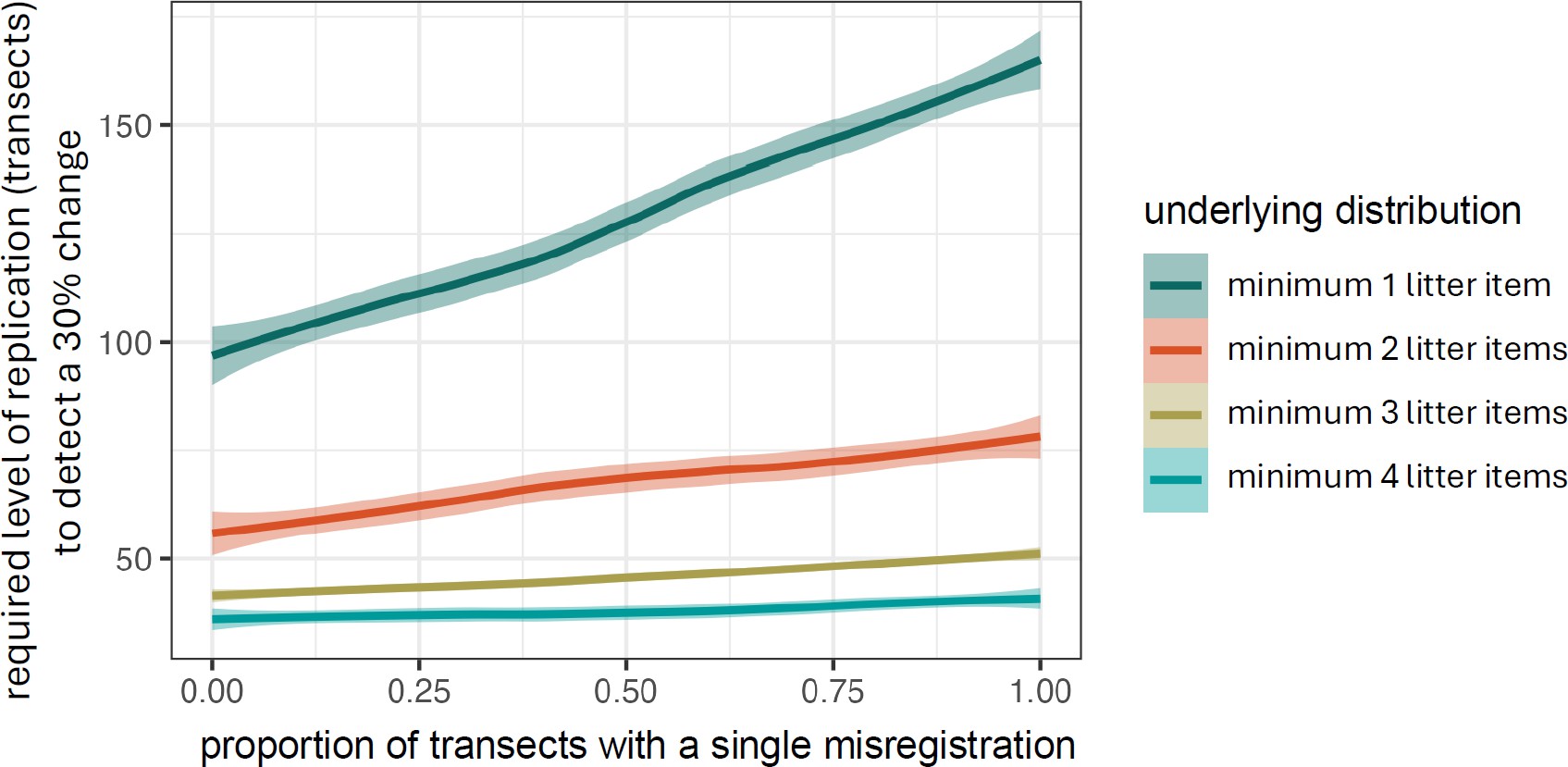
Styrkeanalyser av data fra Mareano-programmet viser at for å oppdage en 30 % endring i søppelmengde med 80 % sikkerhet, kreves det ved overvåking hvert 5. år av mellom 47 og 132 transekt per havområde, avhengig av terskelverdier og søppeltetthet. Det anbefales å overvåke med videotransekt hvert femte år på et tilstrekkelig antall stasjoner (≥3 søppelbiter) i hvert område (totalt 55 transekt per område). For å kunne påvise endringer i søppelmengde, anbefales det å gjenbesøke transekt fra Mareano-programmet som allerede har registrert tre eller flere søppelenheter. I områder hvor tidligere kartlegging av søppel mangler, anbefales det å supplere med stasjoner i områder med høy sannsynlighet for søppelansamling. En ny styrkeanalyse bør gjennomføres etter første datainnsamling for justering av overvåkingsopplegg. For hvert forslag må det beregnes noe høyere kostnader første år, da man må forvente større innsats for å identifisere transekt med ≥3 søppelbiter. I forslaget til overvåkinsprogram er kostnad estimert for en runde med undersøkelser. Vi anbefaler 5 års mellomrom mellom hver runde.
Forslag til overvåkingsprogram:
Minimumsløsning
Kyst: Det anbefales å kombinere gjenbesøk av transekt der det tidligere har vært registrert tre eller flere søppelenheter per transekt med nye transekt i oppsamlingsområder hvor man kan vente lik eller høyere tetthet per transekt.
Oppsamlingsområder inkluderer fjordområder som ligger nært befolkningstette områder som byer eller tettsteder, nært havner, i kystnære marine daler, fjordområder nær kilder, områder nært elveutløp. Vi anbefaler at minst 55 transekt overvåkes hvert 5. år totalt for kyst. Omtrentlig kostnad: Kr 833 000,- + Kr 100 000,- til rapportering.
Hav: For å detektere mulige endringer i oppsamlingsområder til havs foreslår vi at alle tre forvaltningsplanområdene blir slått sammen til ett havområde og at transekt i Mareanos database med tre eller flere søppelenheter gjenbesøkes på samme posisjon som tidligere. Dette vil eliminere behovet for å søke etter nye akkumulasjonsområder til havs som representerer store besparelser. Vi anbefaler at 55 transekt overvåkes hvert 5. år totalt for minimumsløsning hav. Omtrentlig kostnad: Kr 5 212 000,- + Kr 100 000,- til rapportering.
Samme som minimumsløsning for kyst og hav (110 transekt), men i tillegg anbefales det at sårbare naturområder overvåkes på 55 lokaliteter. Disse inkluderer områder med høy tetthet av sårbare arter, f.eks. korallrev, korallskog, sjøfjærsamfunn, ålegrasenger og svampområder. Slike sårbare habitater, spesielt korallrev, har en kompleks romlig struktur som i tillegg til å være habitat for en mengde andre arter også fungerer som «feller» for søppel. Det er vanlig å finne tapt fiskeutstyr (line og garn) på korallrevene. Typen søppel vil være avgjørende for skadepotensialet. For eksempel vil spøkelsesfiske på grunn av tilstedeværelse av tapte fiskeredskaper som teiner, garn etc. kunne være skadelig for sårbare arter i et område. Det vil måtte gjøres styrkeberegninger basert på første runde innsamlet data for å avgjøre hvor mange transekt som er nødvendig for å detektere en 30 % endring med 80 % sannsynlighet. Omtrentlig kostnad: Kr 7 447 000,- + Kr 200 000,- til rapportering.
Fullskala oppsett:
For å kunne detektere en 30 % endring i hvert av de seks områdene, Skagerrak–Nordsjøen, Norskehavet og Barentshavet og kystregionene innenfor med 80 % sannsynlighet, anbefales det besøk på 55 transekt i hvert område (hav + kyst) og 55 i sårbare områder hvert 5. år. Det anbefales å ta utgangspunkt i de allerede kjente lokasjonene i hvert havområde som tilfredsstiller kravene, og supplere med flere stasjoner gjennom fokuserte søk i områder med høy sannsynlighet for søppelansamling.
I kystnære strøk vil typer kilder og tilførselsrater kunne variere mellom regioner, og det anbefales i en fullskala løsning å ta hensyn til dette ved å dele kysten i regioner der det innhentes et tilstrekkelig antall lokasjoner i hver region. Det anbefales at regionene tilsvarer havområdene Nordsjøen/Skagerrak, Norskehavet og Barentshavet.
Med utgangspunkt i at overvåkingslokalitetene som har høy nok tetthet av søppel (≥3 søppelbiter) vil totalt antall transekt som skal gjenbesøkes hvert 5. år være 385. Dette kan nedjusteres med økt kunnskap om søppelmengder i kyst- og havområder hvor tidligere observasjoner er få. Omtrentlig kostnad: Kr 10 820 000,- + Kr 250 000,- til rapportering.
Preface
This report has been funded by the Norwegian Environment Agency and is written in collaboration between the Institute of Marine Research, Salt and Runde Research. The contact person at the Norwegian Environment Agency has been Inger Lise Nerland Bråte. We would like to thank Inger Lise Nerland Bråte for her valuable feedback throughout the process and Kjell Bakkeplass for his assistance with maps and figures. The project managers were Lene Buhl-Mortensen and Bjørn Einar Grøsvik.
The present report is an english translation of the original report:
Buhl-Mortensen, L., Haarr, M.L., Vabø, Ø.S., Thorbjørnsen, S.H., Rydsaa, J., Buhl-Mortensen, P., Vickery G., Smedbold, E., Grøsvik, B.E. 2025. Suggestion for national monitoring of seabed litter in Norway, Rapport fra havforskningen 2025-7, ISSN:1893-4536, 73 Pp.
Summary
Several types of equipment can be used to monitor litter on the seabed, including drop cameras, ROVs (Remotely Operated Vehicles), and AUVs (Autonomous Underwater Vehicles). Drop cameras and video rigs are cost-effective and can cover large areas but have limited flexibility for detailed inspections. ROVs offer greater freedom and can stop for closer examination but are more expensive and dependent on weather and currents. AUVs are efficient for covering large areas quickly and can capture high-resolution images, but they are costly and technically demanding.
Litter is recorded in the field with quality checks of uncertain identifications conducted later after field surveys. Object detection using artificial intelligence (AI) will become efficient once detection algorithms are developed. Given the low densities of litter in Norwegian waters, the most cost-effective method today is direct field recording, requiring trained personnel to perform the work. When relevant AI technology is developed, litter could be automatically detected with quality control by trained personnel.
Seabed litter is generally most prevalent near the coast and at intermediate depths, with plastic, particularly fishing-related plastic (such as ropes and nets), being the dominant category. Other accumulation areas include marine valleys, troughs, and canyons. The Mareano program has mapped litter since 2006, showing that plastic accounts for 64% of all litter, with the highest density at depths between 400–1000 meters. Rivers significantly contribute to plastic pollution, especially plastic from agriculture, such as silage wrap, which often accumulates near river mouths. Through annual ecosystem surveys, the Institute of Marine Research (IMR) also records litter as bycatch in bottom trawls in the Barents Sea and North Sea. This litter mainly consists of fishing-related waste, such as nets and nylon ropes. The extent of lost fishing gear and "ghost fishing" in coastal areas is uncertain, but data from the Directorate of Fisheries and the IMR indicate it is significant.
Power analyses of data from the MAREANO program show that detecting a 30% change in litter quantities with 80% certainty requires 47–132 transects per sea area annually, depending on threshold values and litter density. It is recommended to monitor with video transects every five years at a sufficient number of stations (≥3 litter items) in each area (a total of 55 transects per area). To detect changes in litter quantities, transects from the MAREANO program that have already recorded three or more litter items should be revisited. In areas where previous litter mapping is lacking, additional stations should be added in locations with a high likelihood of litter accumulation. A new power analysis should be conducted after the initial data collection to adjust the monitoring approach. For each proposal, slightly higher costs are expected in the first year due to the effort needed to identify transects with ≥3 litter items. For the estimated cost of monitoring program, we have given estimates per round of investigation. We recommend new investigation every 5 years.
Proposals for Monitoring Programs:
Minimum Solution:
Coast:
Combine revisiting transects with ≥3 waste items previously registered and adding new transects in areas with similar or higher expected waste density. Focus on fjords near urban areas, ports, marine valleys, river outlets, and other waste-accumulation zones. Monitor at least 55 transects every 5 years.
Estimated cost: NOK 833 000 + NOK 100 000 for reporting.
Ocean:
Revisit transects in the MAREANO database with ≥3 waste items in the same positions as before, across all management areas combined into one. This avoids the need to search for new accumulation areas. Monitor 55 transects every 5 years.
Estimated cost: NOK 5 212 000 + NOK 100 000 for reporting.
Total minimum solution (Coast + ocean) NOK 6 045 000 + NOK 200 000 for reporting
Intermediate Solution:
In addition to the minimum solution (110 transects), monitor 55 locations in vulnerable habitats like coral reefs, seagrass meadows, and sponge areas. These habitats are both habitats for species and "traps" for waste like lost fishing gear. Data from the first monitoring round will determine the number of transects needed to detect a 30% change with 80% confidence.
Estimated cost: NOK 7 447 000 + NOK 200 000 for reporting.
Full-Scale Program:
To detect a 30% change in six areas (Skagerrak/North Sea, Norwegian Sea, Barents Sea, and coastal regions) with 80% confidence, revisit 55 transects in each area every 5 years, plus 55 in vulnerable habitats. Use known locations with ≥3 waste items and expand with targeted searches in high-accumulation areas. Coastal regions should account for local waste sources and rates, divided into regions corresponding to the sea areas.
Total transects: 385 every 5 years (adjustable with improved knowledge). Estimated cost: NOK 10 820 000 + NOK 250 000 for reporting.
1 - Introduction
The Norwegian Environment Agency is considering increasing its monitoring of macro-litter, including plastic on the seabed. Internationally, litter items from the seabed have been recorded since 1992, with seabed litter larger than 2.5 cm being collected and recorded as part of the ICES Bottom Trawl Survey as an additional parameter for assessing fish stocks (Galgani et al., 2000). There are several aspects of this monitoring that are not optimal, such as the fact that the surveys are not planned with waste monitoring as their main focus, and data collection is carried out via bottom trawling, which has a negative environmental impact. Therefore, there is an increasing use of image-based monitoring of the quantity and composition of bottom waste. Although there are also limitations to non-invasive monitoring, the Norwegian Environment Agency wants any future monitoring of litter on the seabed to be based on image-based surveys, for example using remotely operated underwater vehicles with cameras and image analysis.This report is in response to a request from the Norwegian Environment Agency to develop a proposal for a national monitoring system for litter on the seabed. It contains an assessment of the appropriate number of monitoring locations, collection frequency, methodology for data collection and analysis, and a customised pipeline for data management. An assessment and recommendation are provided for specific areas that are suitable for monitoring seabed litter (e.g. ports, fjords, coastal areas, exposed seas, etc.) with associated adjustments in terms of methodology. The report provides a recommendation on the procedure and costs for the selected monitoring design that corresponds to the following objectives:
Contribute national data to OSPAR reporting
Identify types and quantities of litter (per area) on the seabed, e.g., sorted according to OSPAR's litter categories.
Document the development of quantities and types of litter items on the seabed on a national scale over time.
Document any differences in the quantities and types of litter items on the seabed between geographical areas.
Assess whether the accumulation areas coincide with vulnerable natural areas.
Document important sources of litter entering the marine environment.
Identify any accumulation areas and any characteristics that affect the accumulation of seabed litter, such as topography, current conditions, etc.
The proposals are based on previous surveys of litter on the seabed, including the MAREANO project (Buhl-Mortensen et al., 2024) and recommendations made through work under the AMAP programme (Grøsvik et al., 2023). To ensure comparable data, it is important to use standardised categories of litter. Since 2023, MAREANO has used the protocol from ICES WGML (Appendix 1).
The main categories in the ICES and OSPAR systems are (ICES, 2022):
A Plastic
B Metal
C Rubber
D Glass and ceramics
E Natural products, including processed wood, paper and cardboard
F Miscellaneous, including clothing/textiles
In a monitoring programme, it is also recommended to add ‘fishing gear’ as a separate item to get a better overview of its presence.
Three different monitoring intensity levels have been developed based on the request from the Norwegian Environment Agency:
Full-scale solution: Provides detailed information on the quantities and types of litter on the seabed at regional level, for different types of water or coastal sections (minimum for the Skagerrak, North Sea, Norwegian Sea and Barents Sea regions).
Downscaled solution: only priority areas with high accumulation potential are included, such as ports, fjords or vulnerable natural areas (e.g., spawning grounds).
Minimum solution: the number of stations is reduced to a minimum, but the monitoring can be used to identify sources and accumulation areas, even though the data will be subject to greater uncertainty. The size of the change over time/place that can be detected as statistically significant with the minimum solution must be described.
2 - Monitoring technology
To monitor macro-litter on the seabed, drop cameras, ROVs, AUVs and other technology can be used, depending on the budget set for the surveys. Underwater monitoring technology is constantly changing, with opportunities for more cost-effective monitoring in the future. The choice of equipment should be considered based on operating depth, desired accuracy, conditions (coastal and ocean environments may require different equipment), and available equipment (Table 1, Table 2).
2.1 - Drop camera and tethered video rig
Drop cameras and towed video rigs represent cost-effective solutions for monitoring the seabed. However, these systems have limitations when it comes to examining litter and other objects more closely. Drop cameras/ video rigs are towed behind the vessel and are well suited for conducting transects of a specific length and direction. The video signal is transmitted in real time to the boat, enabling continuous monitoring and manipulation of the equipment up and down the water column as depths change or obstacles are encountered along the seabed. When using a simple drop camera, there is little opportunity to stop and examine objects more closely, while video rigs can be parked for closer examination of specific objects. However, it does not have the same mobility for conducting closer investigations from multiple angles as, for example, an ROV.
When using a video rig and drop camera, care must be taken not to drag the rig along the seabed before parking for surveys, as this can stir up sediments that can impair visibility. It may therefore be advisable to maintain a low speed. To avoid stirring up sediments when parking the rig, skis can be mounted on the video rig. Several cameras can also be mounted on the rig to expand the field of view and thus cover a larger area. For example, one camera can be used to point forward and two to the side.
In shallow water, the boat's position can be used to determine the position of the drop camera and rig, and with the help of the boat's chart plotter, it is possible to navigate the desired length of transects with a high degree of accuracy. In deeper water (>100 m), the difference between the boat's position and the position of the video rig or drop camera becomes greater. In such cases, it is advisable to use underwater positioning equipment.
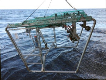
The Institute of Marine Research uses the Chimaera video rig, which is equipped with several video cameras, laser pointers for measuring size, transponders for positioning and CTD (conductivity, temperature, depth).
This can be parked on the seabed for detailed investigations. Chimaera is best suited to seagoing vessels with ample deck space. It is used by Mareano for visual mapping of the distribution and abundance of species, sediments, traces of bottom trawling and marine litter (Figure 1). The rig is equipped with two video cameras (both high and standard resolution), transponders (for depth measurement and geographical positioning), lasers (for image scaling), altimeters (height above the seabed) and Seaguard probes (CTD and current meters).The video rig is towed behind the vessel at a maximum speed of 0.7 knots and is controlled by a winch operator who maintains a near-constant height of 1.5 m above the seabed. Geopositioning of the video rig is performed using a hydroacoustic positioning system (Simrad HIPAP and Eiva Navipac software) with a transponder on the video rig. This system provides a positional accuracy of approximately 2% of the water depth. The videos are stored on hard drives on board the vessel.
Costs: The most affordable drop cameras for use in shallow water cost NOK 15,000–25,000, while slightly more expensive drop cameras can reach depths of 200 metres (NOK 80,000–100,000 including extra lighting). The rental market for such systems is limited.
Advantages: Cost-effective, especially for shallower areas (<100 metres deep).
Disadvantages: Limited possibility for detailed inspection of objects using a single drop camera. This will be somewhat better with a tethered video rig. Less suitable for deeper waters without advanced positioning equipment. Limited possibility to examine objects from multiple angles.
Figure 1: The video rig ‘Chimaera’ equipped with several video cameras, laser pointers for size measurement, transponders for positioning and CTD.
2.2 - ROV
ROVs provide greater freedom to examine objects more closely for reliable identification of debris. In addition, an ROV can be equipped with advanced accessories such as sonars, manipulators and more, which significantly expand its range of applications. ROVs are available in a wide price range, from affordable models costing a few thousand pounds to advanced work ROVs costing millions. If you need to examine areas shallower than 200 metres, especially in sheltered fjords and coastal areas, an affordable ROV will often suffice. There are several suppliers of underwater drones in the price range of NOK 80,000–250,000 that work well at depths of up to 200 metres. As these may have less engine power than the larger work ROVs, you will be more dependent on good current conditions. It is important to ensure that the ROV is equipped with a good video camera (HD or higher resolution) and good lighting for identifying objects. Alternatively, an additional camera, such as a GoPro, can be mounted if the built-in camera does not meet the image quality requirements.
If you are planning a monitoring programme where accurate positioning is important, you will need good positioning data. Underwater positioning can be done acoustically or with internal loggers. Several suppliers offer DVL (Doppler velocity logger) and USBL (ultra-short baseline) for positioning, but this makes the ROVs more expensive. It is also possible to rent USBL systems separately. DVL will be less accurate in positioning due to drift in the system. The USBL system combines a transponder attached to the ROV and a transducer attached either to the side of the boat, integrated into the boat, or in a cable hanging from the boat if the ROV is at greater depths. This system is more accurate than a DVL, but significantly increases the cost. It is possible to rent such systems.
Depending on the monitoring methodology, the exact position is not necessarily important, but the length of the transect and the visibility range are cruical factors in order to estimate the amount of litter per m2. In this case, a DVL will be more affordable and useful. Alternatively, you can note the start and end points for the ROV and calculate the distance between these points.
The accuracy of the start and end points deteriorates the deeper you go, and at depths greater than 50–100 metres, you should have at least a DVL or similar positioning system. When revisiting previously surveyed video transects, especially in challenging environments (large waves) or deeper areas (>100 metres deep), underwater positioning by USBL should always be used to achieve sufficient precision.
In coastal areas and fjords, and when using smaller ROVs, surveys can be conducted from small boats, which makes the operation more cost-effective. It is advantageous for the boat to have a positioning system so that it can remain in position while the ROV dives down to the starting point.
For deeper waters (>200 metres) or in more exposed sea areas, it is most appropriate to use work-class ROVs. These require larger vessels with more equipment. There are many companies that rent out ROV services and provide boats, ROV pilots and crew. Several of these companies also offer to conduct surveys in the field, while a responsible professional monitors a live stream from the ROV via Teams or similar services. These ROVs are more stable and are suitable for use offshore and at greater depths in fjords and coastal areas. They are usually equipped with sonar, a USBL positioning system, and can be equipped with a manipulator (claw), etc.
For deep-sea operations, ROV services are offered by several companies, including boats, ROV pilots and crew. Surveys can be carried out in the field with professionals following the live feed from the ROV via platforms such as Teams. Such services typically cost NOK 40,000–100,000 per day, depending on the location and duration of the assignment. Mobilisation and travel costs are additional and depend on the distance the operators have to travel.
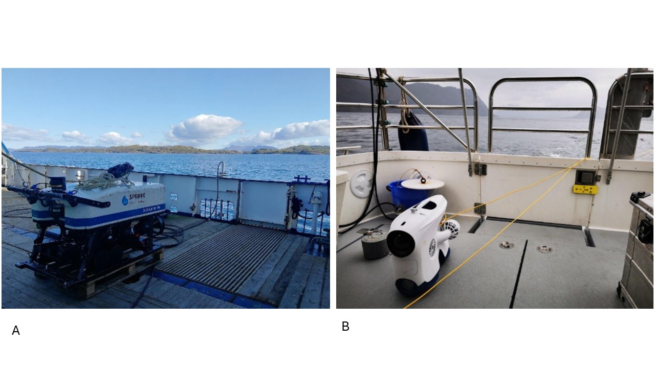
Costs: The most affordable ROVs can cost between NOK 10,000 and NOK 250,000, while the most expensive ones cost several million kroner. Rental prices often range from NOK 1,000 per day to around NOK 4,500 per hour (and more), depending on what is needed to carry out the surveillance (Figure 2).
Advantages: Great freedom of movement for investigations, which can provide detailed examinations of objects. Wide price range. Can be carried out cheaply under certain conditions and at some depths.
Disadvantages: Can be more difficult to stay on course without a positioning system. Expensive at greater depths or in demanding conditions when large ROVs are needed.
Figure 2: Examples of different price ranges for ROVs. The ROV in image A) will cost around NOK 4,500 per hour (excluding mobilisation costs, etc.; estimate for 2024), while the ROV in image B) will cost around NOK 500–2000 per day (estimate for 2024).
2.3 - AUV
An AUV (Autonomous Underwater Vehicle) is (often) a torpedo-like craft with a propeller that travels underwater following a pre-programmed pattern. It can be programmed to maintain a fixed distance from the seabed, making AUVs an ideal platform for photographing the seabed. During data processing, the still images are assembled into a photo mosaic that is linked to the AUV's position. It is possible to communicate with the AUV underwater via acoustic modems, as well as to track its position using the same technology. A height of 4 metres above the seabed is often optimal for identifying species and objects. AUV operations usually take place at a speed of around 4 knots.
In addition to photography, AUVs can be equipped with side-scan sonar, which provides echo images of the seabed. These have relatively high resolution and can be used to identify objects such as ropes, pots and bottles, but not smaller pieces of rubbish.
AUVs are more expensive, with prices ranging from a few hundred thousand for very simple models to tens of millions for the more advanced variants.
Advantages: Covers large areas efficiently. Detailed images can be taken and advanced sensors such as side-scan sonar can be used.
Disadvantages: Limited suitability in rugged terrain. Most AUVs require detailed depth data to plan their route. Advanced models and their operation are costly. Operation and analysis require specialised technical expertise, and software for producing photo mosaics can be difficult to use. No possibility to stop and examine any rubbish from multiple angles.
2.4 - Methodology
When operating a drop camera, tow camera rig and ROV, it is crucial to maintain a moderate speed tthrough the survey area. High speeds can make it difficult to identify both litter and litter types, both for personnel and artificial intelligence (AI), due to the risk of unclear and distorted images.
Experience from the Mareano mapping programme indicates that at speeds above 0.7 knots, it is difficult to identify smaller objects. The width of the field of view per camera (controlled by the angle of the lens and height above the seabed) is also a factor that can limit image quality. The width of the field of view should not exceed 4 metres. The height above the seabed and the camera's angle of incidence must be adjusted to provide a good overview, while at the same time ensuring that the field of view is not so large that objects on the seabed become blurred. Measures to ensure good images are particularly important in fjords with high sedimentation rates, as the litter here may be partially covered by sediment.
It is recommended to add laser pointers to the survey equipment to measure the size of litter and the image field that is analysed manually or by AI. Lasers can provide valuable information about litter density in a transect. Ideally, lasers with two or four points with a known distance between them should be used. Alternatively, stereo or mono images can be used for size calculations, depending on the number of cameras available.
The season also plays a role in how easy it is to find litter in shallow areas (0–40 metres). In these areas, it is recommended that surveys be conducted in winter when macroalgae are at their smallest and plankton blooms have not yet occurred. In areas north of Stad, October to February is ideal, while south of Stad, November to early February is preferable for mapping such shallow areas. It is also recommended to avoid areas near major river outlets after rainfall, as runoff can impair visibility.
Depth
Necesserytechnology
Timeconsumption
0– 50
Simple ROV, drop camera or tow camera rig.
Short time due to depth.
50- 100
Simple ROV, drop camera or tow camera rig. Good lighting is essential.
Slightly longer time due to depth.
100– 200
Simple ROV, drop camera or tow camera rig. Good lighting is essential. In strong currents and challenging environments, larger ROV is required.
Slightly longer time due to depth.
200– 500
Larger ROV, drop camera, towed camera rig, or AUV required. Good lighting is necessary.
Time-consuming to obtain observations in the deep sea and position data can be challenging.
500– 1000
Larger ROV, drop camera, towed camera rig, or AUV required. Good lighting is necessary
Time-consuming to obtain observations in the deep sea and position data can be challenging.
1000+
Larger ROV, drop camera, towed camera rig, or AUV required. Good lighting is necessary.
Time-consuming to obtain observations in the deep sea and position data can be challenging.
Table 1: Schematic overview of relevant methods and technologies that can be used to collect image material.
Instrument
Advantages
Disadvantages
Costs (NOK)
Areacover (estim. m2)
Drop camera
Affordable. Easy to follow transects. Good positioning quality. Good image quality, can be improved with external cameras.
Lack of freedom to move around and stop at interesting discoveries
Buy: 10 000- 100 000 Rent(perday): 500- 2000
5- 7
ROV small model
Affordable. Can be used from open boats down to depths of 200 metres. Decent image quality that can be improved with external cameras. Freedom of manouvering.
Often more difficult and expensive with positioning equipment. More vulnerable to poor weather conditions and strong currents.
Buy: 10 000-400 000. Rent(perday): 1000- 2000
5- 7
ROV work class
Good image quality. Can go deeper than 200 metres. More robust and more manoeuvrable in difficult conditions. More options for connecting equipment. Work can be done from the office. Positioning equipment Freedom of manouvering.
Expensive, and must be done from a boat with special equipment.
Rent(perdag): 40 000-150 000 Buy: From 20 000 depending on how deep it will be used, as well as additional equipment.
5- 7
Towed camera- rig
Image quality depends on the camera selected. Can be used from smaller boats, but requires a winch and an area to monitor the video stream. Preferably down to a depth of 200 metres. Can be stopped when a find is made. Positioning equipment can be attached.
Lacks freedom to move around, but can stop at interesting discoveries.
Rent: Limited rental market. Buy: from a few hundred thousand to millions.
AUV
Covers larger areas in less time.
Expensive and difficult to lay routes near the bottom in hilly terrain.
Rent: limited market for rentals.
Mosaic. Width of mosaic: 2-5 m
Table 2: Schematic overview of relevant instruments that can be used to collect image material.
2.4.1 - Cost estimate
Equipment costs for ROVs vary and depend on factors such as brand, depth rating and camera (Table 3). The rental price of ROVs suitable for use in shallow water varies depending on who you rent from, and for most people it will be most natural to purchase such an ROV if they do not already have one, as the price is so low.
Modell
Price(excl. VAT) (NOK)
Rent(estimate per day) (NOK)
Rateddepth
Camera
Light
Chasing (flere modeller)
36 000– 75 000
1000–2000
150– 200 meter
12 mpx, 4K Sony CMOS + EIS anti-vibration
2x2000 or 2x4000 lumen led light.
Fifish
16 000– 75 000
1000–2000
100– 200 meter
12 mpx, 4K
2x4000 lumen/4x3000 lumen
BluEye
55 000– 250 000
1450
150– 305 meter
2K
3300 lumen
BlueRobotics
120 000– 230 000 NOK
1000–2000
100– 300 meter
1080 HD
4x1500 lumen
Deep Trekker DTG3
Ca. 130 000
1000–2000
< 200 m
1080 HD
1000–54000 lumen
Table 3: Costs and specifications for ROVs suitable for use in shallow water (<200 metres).
3 - Image analysis
Most surveys and maps of marine litter on the seabed are based on trawl data. This also includes the maps published by the European Marine Observation and Data Network (EMODnet) (Galgani et al., 2022) and ICES (ICES, 2022). In areas that are inaccessible to trawling, other methods have been used, such as diving surveys, USVs (Unmanned Surface Vehicles), towed underwater cameras (TUCs), AUVs and ROVs (MSFD Technical Group on Marine Litter, 2023). The following description deals with the analysis of video and images from TUC, AUV or ROV.
3.1 - Manual image and video annotation
Video analysis: CampodLogger and Seabed Field Observer software. Both programmes were developed at IMR, are publicly available and can be used to take notes on fauna, seabed types, signs of fishing activity, the presence of litter and local geological seabed features during video recording. Along with the notes taken while the transect is being carried out, these programmes also record navigation data (date, UTC time, position) and depth for the boat and video rig.
The observation width of the video image is normally 2–4 m of the seabed and is used together with distance (from position data) to calculate the area covered by the video transects and the density (n/km2) of litter for video transects (see Buhl-Mortensen & Buhl-Mortensen, 2017, 2018 for more information on the methods).
Litter items should be recorded in categories used by ICES (ICES, 2022) (Appendix 1). This standard has been developed by the ICES Working Group of Marine Litter (WGML) and is also used by OSPAR as the standard for reporting litter on the seabed.
Calculation of litter quantity: Raw data from video observations may be the number of observations per video transect. The density of different litter categories will be standardised according to the length of each video transect to provide number/100 m of seabed length and items/km². The area observed for each video transect is calculated by multiplying the length of the transect by the average width of the field of view. Number of observed items per square kilometres (km²) is a unit that ensures comparability with both international publications and previous work (see Buhl-Mortensen & Buhl-Mortensen, 2017 & 2018).
As only macro litter will be examined during manual surveys, this will take relatively little time. Mareano data, reported by Buhl-Mortensen et al. (2024), show that there is generally very little litter on the seabed on the continental shelf and in other deep sea areas. This data is based on field recordings made using the Campodlogger logging programme. A cost-effective approach would be to use only post-analysis of video recordings to study uncertain observations from the field, where it is possible to pause the recording and take still images to zoom in on details.
If entire videos are to be annotated in more detail after the expedition, the costs for this can be calculated based on the following assumptions: Assuming that the video can mainly be played back at normal speed during analysis, and that one is traveling at 0.7 knots while maintaining a distance from the bottom that gives a width of 3 meters, one will be able to see approximately 0.36 meters per second of film, giving 1.08 m observed (3 m*0.36 m = 1.08 m2). If you add a little time for closer examination of the plastic and identification, you can on average manage 0.25 meters of transect per second corresponding to 0,75 m2 (3m*0,25m = 0,75m2 ) per second.
100 m/0.25 m/s = 400 seconds ≈7 minutes
Based on a transect of 100 meters, this will take approximately 7 minutes. At an hourly rate of NOK 1,400, this amounts to approximately NOK 165 per transect (100 meter) and NOK 1.65 per square meter analysed.
Depending on the complexity of the seabed, it may also take longer to complete the transect. To take this into account, one can estimate 10 minutes per 100 meters as an average. Some transects will be filmed more quickly, while others (for example, in complex coral reefs) will take longer to film. At 10 minutes per transect, this amounts to NOK 233 per 100-metre transect and NOK 2.33 per meter analysed. There will also be costs associated with start-up and general operation (recording meta data, etc.). One can therefore add 10 minutes of operation per transect (233 NOK).
The costs for 100 meter will be: (2.33 NOK/m*100 m) + 233 NOK = 466 NOK.
With a distance to the bottom that provides a transect width of 3 meters 300 m2 can be mapped to a cost of NOK 0.77/m. We recommend different transect lengths near the coast and on the continental shelf/offshore, depending on the depth and type of monitoring area (harbour, fjord bottom, open sea and river mouth). The calculations in the strength analysis (Chapter 5) are based on MAREANO data, where the longest transect length is 750 metres. This length is recommended for transects on the continental shelf/offshore. In some cases, it may be difficult to place a 750-metre transect in coastal areas. In shallow areas (<100 metres), the time it takes to lower and raise monitoring equipment is relatively short, but in some cases it may be difficult to place a 750-metre-long transect and several shorter ones must be taken.
3.2 - Image processing with artificial intelligence (AI)
A number of AI models have been used to detect benthic marine litter from AUV data. Successful model developments include Faster RCNN, ResNet, SVM, and several YOLO versions, with average accuracy ranging from 55% to 83% (Deng et al., 2023; Politiokos et al., 2021; Xue et al., 2021; Jalil et al., 2023; Chin et al., 2022; Bajaj et al., 2021). The quality of the models depends on several factors: the size of the dataset, the variation in the training data, the image quality and the type of litter to be detected. In shallow areas, the models are also affected by differences in light intensity; if the model is trained on images with a lot of light, it can be difficult to use it on data with little light (Chen et al., 2020). At this point, it is the YOLO models (within the Ultralytics Python package) that typically give the best results.
All models used fall within the category of ‘neural networks’ under the broad term ‘AI’. This mainly concerns object detection, but there are also a few examples of instance segmentation (Hong et al., 2020; Đuraš et al., 2024). Both of these approaches identify several different litter objects within each image or video frame. The difference is that in object detection, the model draws a square bounding box tightly around objects, while in segmentation, it draws a polygon precisely around the object's boundaries. Segmentation provides more accurate information about an object, but the time required to label objects is significantly longer. It is possible to extract size estimates from both methods if filming is done in stereo.
For the most effective mapping of marine litter, one can start by using existing data to estimate ‘hot spots’, areas with an expected high density of litter. This can also be combined with modelling probable hot spots based on, for example, supply points (rivers, ports, cities) and current models. Modelling methods that can be used include random forests (Cau et al., 2024) and more complex CNNs (Franceschini et al., 2019). Once areas have been identified, a suitable methodology for data collection can be selected. The data collected can also be used to inform and validate the predictive models.
As mentioned earlier, different types of marine litter are categorised in an EU directive by the Marine Strategy Framework Directive Technical Group on Marine Litter (Fleet mfl., 2024).
This list summarises the classifications used by OSPAR, ICES and other leading organisations, where litter is classified according to material, type and size. Regardless of the observation methodology, classification should be carried out in accordance with this list to ensure future comparability. This will also be a major advantage in terms of being able to reuse AI models. Furthermore, additional categories may be added if deemed relevant to the purpose of the monitoring.
3.2.1 - Image processing pipeline
For mapping and AI analysis of marine litter on the seabed, the following pipeline for video and image analysis is proposed, modified from Politikos et al. (2023):
Data collection. Appropriate methodology for collecting video and image data is selected based on location (coastal, open sea) and depth.
Identify the machine learning task and select the model architecture. The task may be, for example, object detection and/or classification. The resolution, availability and suitability of the collected data are specified to ensure that the data is of sufficient quality to perform the task.
Pre-processing of data. This may include cropping images, such as removing visible parts of the camera rig, and increasing the contrast or brightness (Bancud et al., 2023; Singh et al., 2023).
Data annotation. Objects are identified and annotated. This is an essential part of the process, where the quality of the model is directly dependent on the accuracy of the annotation (Paullada et al., 2021). The categories should be set at the beginning and the data annotated accordingly. The development of tools for data annotation is progressing rapidly. One example is the AI model ‘Segment Anything’ (Meta AI, 2023). There are pre-annotated datasets of images of litter on the seabed that are openly available and can be used to train new models (Example: TrashCan 1.0, Hong et al., 2020), but these can be of varying quality and it is likely that one will also have to use one's own material to ensure representativeness of plastic objects and background/ environment.
The dataset is divided into training, test and validation sets. It must be ensured that there is no overlap between the annotations assigned to each subset, so that the model is trained, tested and validated on different data. The validation set is used to continuously evaluate how well the model performs. The test set can be used retrospectively to test the model on new data.
Data augmentation. By making small and varied changes to data that has already been collected, it is possible to increase the amount of data and, in turn, reduce over-fitting in the model. This means that the same image is entered several times, but with slight changes so that they are slightly different. Examples of changes include distorting, mirroring or rotating the image. The background can also be changed. It is recommended to evaluate the effect of this on each class (Bhalla et al., 2024).
Model training and fine-tuning of hyperparameters . Fine-tuning the parameters optimises the training of the model by, among other things, adjusting how sensitive the model is to different characteristics in the data. It also involves adjusting how many times the model goes over the data, where it evaluates and adjusts itself for each round.
Evaluation and repetition . The model is evaluated. As a minimum, the model's precision and proportion of ‘true positives’ are assessed. This should be done individually for each class, and the average for all classes taken together should also be assessed.
3.2.2 - Cost estimate
The cost of image processing with AI is highest at the beginning, when the model is being developed and trained to acceptable precision. Once the model is ready for use, the operating costs for video analysis will be low, comprising only the costs of servers and CPU hours (processing). When starting to develop the model, it may be useful to contact authors of research articles on the detection of marine litter on the seabed (see examples in Chapter 4.2). You can ask for access to image material with accompanying annotations of litter, which can give you a head start in your own model development. This can, for example, help to detect litter in your own image material, which can then be checked and placed in the correct category. You can also ask for access to the model, but if you do gain access to it, in many cases you will still need to allow time for formatting the data. It will vary whether it is worthwhile to continue working on an existing model trained on other data or whether it is worthwhile to create a new one from scratch. Factors that influence this include what the images look like, for example whether the background is similar, whether the images are taken in the same way (e.g. ROV vs. drop camera) and whether the images have the same image quality.
The time required to achieve an AI model with sufficient precision will vary depending on the type of data to be detected. In the case of litter, the model will have to learn to recognise objects with great variation in shape, colour and size. The speed of development of new models and methodologies for faster model training (such as ‘Segment Anything’ mentioned above) is rapid and is likely to continue. It is therefore possible that the time frame will decrease over time. It is estimated that around 800 hours should be set aside for the development of an AI model for image recognition of litter, from start-up to finished product. The cost estimate then comes to 800 hours x NOK 1,400/hour = NOK 1,120,000. Please note that there is uncertainty associated with this estimate, as it is difficult to estimate the exact time required.
Estimating the costs of field surveys is a complex calculation and involves uncertainty. Some estimates have been made in the calculations, and prices will vary depending on the distance to the stations, the distance that hired consultants and ROV services have to travel, and other factors. Nevertheless, an attempt has been made to provide an insight into the costs in the table below (Table 4). The external rental price for a relatively small boat and ROV in coastal waters shallower than 300 m is estimated at NOK 50,000 per day. The cost of a suitable vessel for coastal and fjord areas deeper than 300 m is estimated at NOK 75,000 per day. The price for ocean-going vessels including ROVs is around NOK 300,000 per day including fuel in 2025.
<300mdepth
>300mdepth
Sum
Costs( NOK)
Monitoringlevel
Transect
Days
Transect
Days
Transit days
Transect
Days
Vessel
Manning/travel
Total
Minimum
Coast
30
3
25
2
3
55
8
525 000
308 000
833 000
Offshore
20
2
35
3
6
55
11
4 400 000
812 000
5 212 000
Total
50
5
60
5
9
110
19
4 925 000
1 120 000
6 045 000
Intermediate
Coast
30
3
25
2
3
55
8
525 000
308 000
833 000
Offshore
20
2
35
3
6
55
11
4 400 000
812 000
5 212 000
Vulnerable ecosystems coast
10
1
15
1
-
25
2
150 000
92 000
242 000
Vulnerable ecosystems offshore
15
1
15
2
-
30
3
924 000
236 000
1 160 000
Total
75
7
90
8
165
15
5 999 000
1 448 000
7 447 000
Full-scale
Coast
110
8
55
3
3
165
14
850 000
524 000
1 374 000
Offshore
60
4
105
7
6
165
17
6 800 000
1 244 000
8 044 000
Vulnerable ecosystems coast
10
1
15
1
-
25
2
150 000
92 000
242 000
Vulnerable ecosystems offshore
15
1
15
2
-
30
3
924 000
236 000
1 160 000
Total
195
14
190
13
36
385
27
8 724 000
2 096 000
10 820 000
Table 4. Estimated time and costs for fieldwork for the three monitoring strategies. The calculations have been made separately for shallow (<300 m deep) and deeper (>300 m) locations. A boat rental rate of NOK 50,000 per day has been used for locations <300 m offshore, NOK 75,000 for locations <300 m offshore, and NOK 400,000 per day for offshore locations. These rates include the rental of ROVs. Crew and travel are specified with the normal trip allowance added.
4 - Review of knowledge: Distribution of litter on the seabed in Norwegian waters
4.1 - Observations on the coast
The Institute of Marine Research, the Norwegian Geological Survey (NGU) and the Norwegian Mapping Authority collaborated on the ‘Marine grunnkart’ project to create detailed base maps of the coastal zone. Using several hydrographic models, grab sampling and multibeam sonar, as well as video footage collected using drop cameras and ROVs, seabed conditions (bathymetry and sediment types), biology and litter have been mapped in the coastal zone. To date, parts of Ryfylke, parts of Møre og Romsdal and parts of Troms have been mapped.
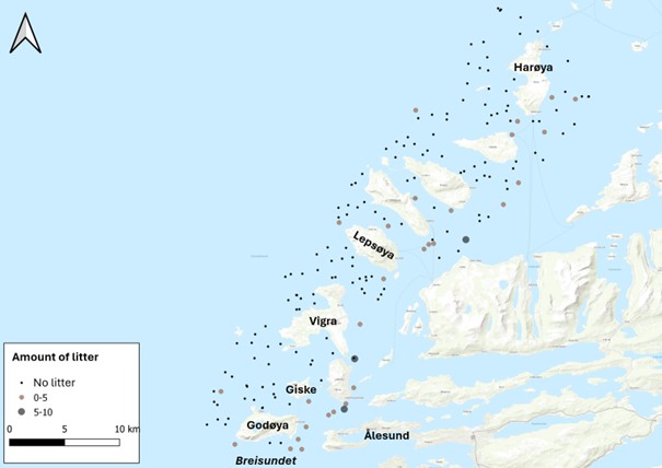
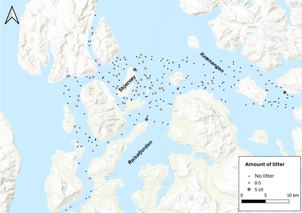
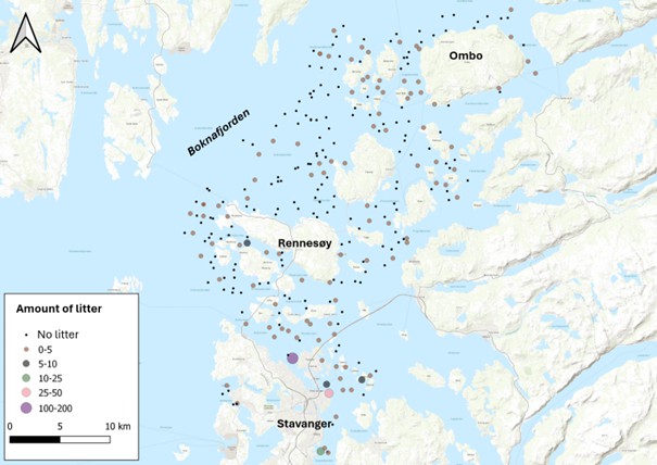
From Ålesund and Giske, the mapping shows that litter is most frequent inshore, on the inside of the Nordøyene islands and most transects in the northern part of Breisundet, as well as near Ålesund (Figure 3). In Nord-Troms, there are many transects with observed litter around the fishing village of Skjervøy – and fewer transects with litter with increasing distance from Skjervøy and the surrounding sounds (Figure 4). In Stavanger, the largest concentrations of litter have been observed around Stavanger city centre (Figure 5).
There are also several transects with observations of litter between the islands west of Ombo.
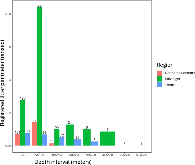
In the areas mapped by Marine grunnkart, the highest number of pieces of litter per metre surveyed is between 50 and 100 metres, and in general the most litter per metre is observed in Stavanger (Figure 6).
Figure 3: Video transects with and without observed litter in Marine Base Map surveys in Ålesund and Giske. Data retrieved from GeoNorge.
Figure 4: Video transects with and without observed litter in Marine Base Map surveys in Northern Troms. Data retrieved from GeoNorge.
Figure 5: Video transects with and without observed litter in Marine Base Map surveys in Stavanger and parts of the Ryfylke fjords. Data retrieved from GeoNorge.
Figure 6: Number of litter observations per meter divided into depth intervals for the three regions of Northern Sunnmøre, Stavanger and Northern Troms. The numbers at the top of the bars indicate the number of transects surveyed in each depth interval in each region. Data retrieved from GeoNorge.
4.1.1 - Litter near river mouths
In order to gain knowledge about the types and quantities of litter transported from rivers into the sea, a survey of litter on the seabed was conducted in 2022 off the three rivers Uskedalselva, Storelva (Omvikdalen) and Rosendalselva in Hardanger (Buhl-Mortensen 2023). The survey was a collaborative project between the Institute of Marine Research and Bergen og Omland Friluftsråd (Bergen and Omland Outdoor Council). The three rivers mainly flow through agricultural areas. Some registration of waste transport in the rivers has been carried out (NORCE 2020), and in some places 10 plastic fragments per 100 metres of river stretch have been reported.
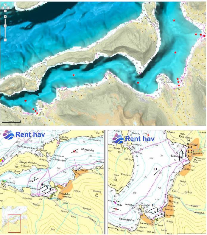
Fourteen locations were selected at varying distances from the river mouths and land, and 11 of these were surveyed. At each location, an ROV line of approximately 300 metres in length was carried out (a total of 13 transects). The positions of the video lines and the amount of litter are shown in Figure 7 and Table 5.
Observed litter
A total of 214 items of litter were recorded, and the quantity and types of litter observed, along with photographs showing examples of the litter observed, is shown in (Tables 6 and 7, and Figure 8). The largest quantity of litter recorded along a transect was 77 items, which corresponds to 230 items per 1000 m2 or 230 000 items per km2.
Figure 7: At the top, a bathymetric map showing the 14 planned ROV locations (red stars), rivers and settlements. Below is the location o fthe ROV lines that were completed with the numbers (1-11) on them, red crosses mark those that were not visited. Details are given in Tables 5-7. Retrieved from Buhl-Mortensen, (2023).
Leaves and branches are deposited closest to the river mouth (zone 1), while large amounts of litter were observed further from land at depths of 24–77 metres outside the river mouth in zones 2 and 3 (see Tables 6–7). The observed litter density ranged from 30,000 to 230,000 litter items per km2 is very high both nationally and internationally. In a European context, a density exceeding 2000 litter items per km2 is defined as a high degree of littering (Pham et al. 2014).
On this basis, a high degree of littering has been documented on all the video lines carried out, and the largest occurrences were due to plastic pieces (fragments approx. 10–20 cm in length) that appear to originate from plastic used around hay bales.
The study shows that the rivers contribute a significant amount of plastic to the fjord, but that much of it ends up on the seabed close to the river mouth. The high figures are representative of the zone outside the rivers and cannot be considered as general values for larger areas of the fjord outside.
Locality
Videoline
Time
Position
Depth
Transect
Litter
Litter
Lat
Long
(m)
(m)
items
km2
Rosendal
1- 1
08:45
59o 59.049
6o 00.287
27,3
150
4
Rosendal
1- 2
09:21
59o 59.085
6o 00.317
14
25
3
Rosendal
1- 3
09:40
59o 59.085
6o 00.317
14- 40
150
9
1-1 & 1- 3
300
13
39000
Rosendal
2
10:09
59o 58.922
6o 00.133
53- 32
300
10
30000
Rosendal
3
10:57
59o 58.894
5o 59.853
77- 40
300
14
42000
Uskedal
4
12:05
59o 55.815
5o 51.076
0,4- 17
300
2
6000
Uskedal
5
12:35
59o 55.847
5o 51.045
24- 56
300
24
72000
Uskedal
6
13:21
59o 55.878
5o 50.937
57- 55
300
26
78000
Storesund basin
7
14:37
59o 56.237
5o 50.614
203- 205
300
12
36000
Lundsvika
8
16:30
59o 57.197
5o 59.144
15- 9
300
2
6000
Lundsvika
9
17:08
59o 57.254
5o 59.120
31- 37
300
30
90000
Lundsvika
10
17:52
59o 57.360
5o 59.287
50- 44
300
77
230000
Deep basin
11
19:02
59o 58.515
5o 59.034
161- 164
300
4
12000
Table 5: Overview of stations outside three rivers in Hardangerfjorden that were visited with ROV in 2022. The table contains position, depth, length of video line and observed litter specified as items observed and calculated as number per km2. The calculation is based on a 300 m video line with an average observation width of 1 m.
Table 6. Overview of stations visited by ROV on September 15th 2022, together with information on depth, seabed conditions, number and type of litter observed.
Zone
Locality
Video
Depth
Litter
Litter
line
(m)
items
km2
Rosendal
1-1 & 1- 3
14- 40
13
39000
1
Uskedal
4
0,4- 17
2
6000
Lundsvika
8
15- 9
2
6000
2-13
17000
Rosendal
2
53- 32
10
30000
2
Uskedal
5
24- 56
24
72000
Storelva
9
31- 37
30
90000
10-30
64000
Rosendal
3
77- 40
14
42000
3
Uskedal
6
57- 55
26
78000
Lundsvika
10
50- 44
77
230000
14-77
116667
4
Deep basin
7
203- 205
12
36000
Deep basin
11
161- 164
4
12000
4-12
24000
Table 7: Overview of litter density as number observed and number per km2 at different distances from the river mouth. 1: in shallow water just outside the river, 2 and 3 further out and parallel to the river mouth, and 4 in the deep basin of the fjord outside (see also map in Figure 7). Figures in bold indicate the average value.
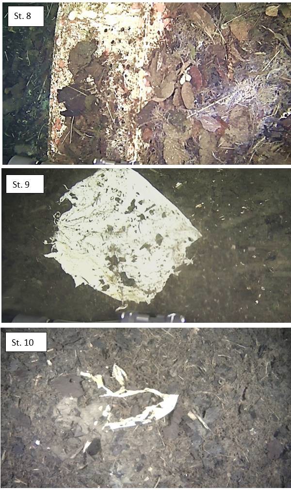
Figure 8: Examples of litter observed at different distances from the river mouth in Lundsvika. Closest to the river (station 8), there was little litter; the photo shows a flower box. Further out in deeper water at station 9, there was a lot of white agricultural plastic packaging. At the furthest point (station 10), pieces of plastic from agricultural plastic packaging were very common. Taken from Buhl-Mortensen (2023).
4.1.2 - Litter on the seabed near beaches with high litter concentrations
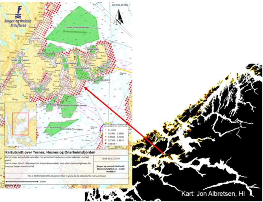
International publications on marine litter estimate that 70–80% of all litter in the sea ends on the seabed. To answer the question: "Is there a lot of litter on the seabed in areas with large amounts of beach litter?" IMR in collaboration with Bergen og Omland Friluftsråd, mapped the occurrence of litter on the seabed around Tysnes island in 2018, funded by the Norwegian Environment Agency (Buhl-Mortensen & Buhl-Mortensen, 2023).
The area was chosen because modelled transport of litter indicates large amounts of litter (Figure 9), and beach clean-ups in the area had documented large amounts of plastic and other litter that probably had accumulated there over a long period of time (Figure 10).
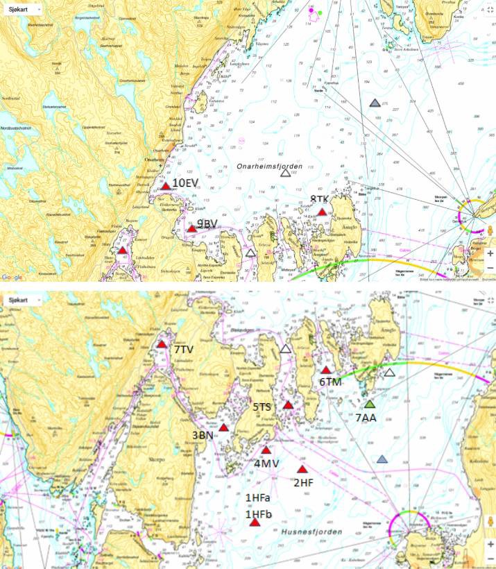
Litter on the seabed was surveyed by boat and ROV rented from Njord Aqua, and a total of 11 dives were carried out at 10 locations (Figure 11). At each station, a 500 m long transect was filmed, covering an area of approximately 1000 m2. The locations visited were located just beyond areas where a lot of litter has been observed on land. Information about position, depth and observed litter is presented in Table 8, and Figure 12 shows a map with positions.
Figure 9: Red dots indicate areas with a high probability of litter stranding, based on the Ocean Current Model (J. Albretsen, Institute of Marine Research). Retrieved from Buhl-Mortensen & Buhl-Mortensen, 2023.
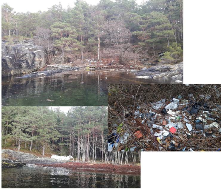
Figure 10: Beach clean-ups have revealed that there is a lot of plastic and other litter on beaches in the area, which has probably accumulated over a long period of time (Photo: B.E. Grøsvik, Institute of Marine Research). Retrieved from Buhl-Mortensen & Buhl-Mortensen (2023).
The study shows a very low incidence of litter on the seabed. Eleven litter items were recorded, six of which were at a station near a key. Litter was observed at only four of the 11 transects (36%). In an earlier study of benthic communities in Hardangerfjorden (Buhl-Mortensen & Buhl-Mortensen, 2014), litter was found at 49% of the 38 locations surveyed, but never in large concentrations. Plastic accounted for a small proportion of the litter.
The results of this study show that there is no correlation between the amount of plastic and litter brought ashore in an area and the littering of the seabed in the vicinity. With the reservation that this is a very limited pilot study, we nevertheless conclude that: it is a light type of plastic and litter that is transported in the upper water layers and ends up on land, while the litter found on the seabed is of a different and heavier type and is supplied from other sources and by other means.
Figure 11: The maps show the 10 locations that were surveyed, marked with red triangles; the station marked with a green triangle had to be abandoned due to strong winds. Planned stations that were not visited are marked with a white triangle. Blue triangles are locations that were surveyed by the "Epigraph" project (Buhl-Mortensen & Buhl-Mortensen, 2014).
Station
Date
Start kl.
Time
Depth (m)
Sediment
Litter items
Litter-category
Comments
1HFa
27.11.
12:22
00:28
102- 131
Bedrock
1HFb
27.11.
12:57
00:49
105- 129
Mud
2HF
27.11.
14:13
00:21
180- 182
Mud
Cable severed, but ROV saved
3BN
27.11.
15:20
00:30
56- 65
Mud
3
Glove, Line (nylon), Rubbish
4MV
27.11.
16:38
00:10
13- 36
Gravely Mud with rocks
1
Bottle
5TS
28.11.
10:04
00:17
12- 35
Bedrock, Gravel Mud w rocks
6TM
28.11.
10:57
00:29
75- 87
Bedrock, Mud
1
Plastic
One piece of litter (plastic hose recovered by ROV)
7AA
28.11.
-
-
-
-
Interrupted due to problems with depth gauge and increasing wind
7TVH
28.11.
13:30
00:26
27- 52
Mud
8TK
28.11.
14:48
00:23
20- 64
Bedrock, Gravel Mud w rock
9BV
28.11.
15:43
00:22
11- 76
Bedrock, Mud, Rocks
10EV
28.11.
16:43
00:24
10- 61
Bedrock, Mud
6
iron, chain, line, strips, barrel ring, wire, iron ring
Table 8: Overview of stations visited, including information about position, depth and observed litter.
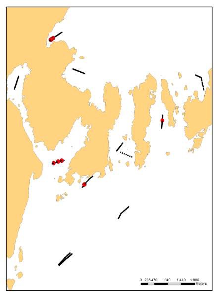
Figure 12: Position of the 11 video transects conducted around Ånuglo, Vestland.
4.1.3 - Overall conclusion on litter distribution in coastal areas
The litter is most prevalent inshore. There are many transects with observed litter around the fishing village of Skjervøy. The highest concentrations of litter are found around towns and in densely populated coastal areas. The highest number of litter items per metre is found at depths of between 50 and 100 meters.
At river mouths, large amounts of litter have been observed some distance from land (50–100 metres) at depths of 24–77 metres. The density of litter has been measured at 30,000–230,000 items per km2.
In agricultural areas, agriculture-related plastic is the most common type of litter. The high waste densities observed in the zone outside the rivers cannot be considered representative of larger areas in the fjord outside, but show that the rivers contribute significantly to the amount of plastic in the fjord, although much of it ends up on the seabed close to the river mouth.
In areas where large amounts of litter have been observed on land, correspondingly large amounts are not found on the seabed. The type of light litter that ends up on land is different from the heavier type normally observed on the seabed, which is contributed from other sources and via other routes.
4.2 - Offshore observations
Offshore, the MAREANO programme is the mapping activity that has most data on the occurrence of litter on the seabed and covers the largest area. MAREANO maps the seabed with a focus on: depth conditions, biodiversity, biotopes, sediment composition, pollutants and traces of human impact. The mapping is non-destructive, as it is carried out using video analysis. Traces of human impact recorded are the presence of trawl marks and litter on the seabed, including lost fishing gear. Plastic finds are categorised, as far as possible, according to relevant protocols (OSPAR and ICES protocols) so that the observations can be compared with other results, such as beach litter. Mareano has recorded observed litter since mapping began in 2006, and an overview of data up to autumn 2023 is presented in a report (Buhl-Mortensen et al., 2024). In total, this material comprised 3,421 video transects, each covering a length of 700 m (until 2017) or 200 m (after 2017).
4.2.1 - General distribution in Norwegian waters
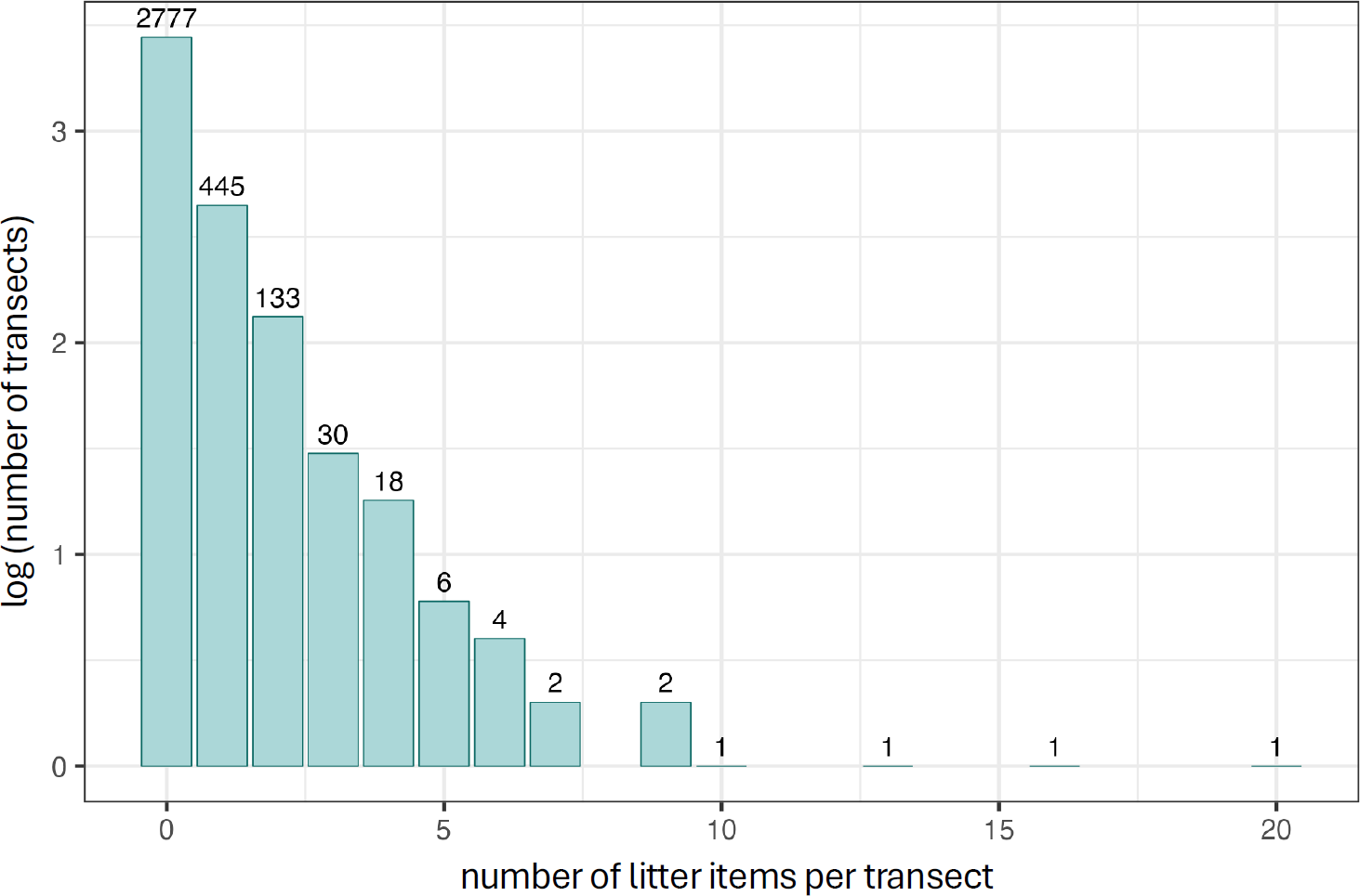
Most of the sites surveyed by Mareano have no litter, and in total, litter has been observed in 18.9% of all 3,421 video transects surveyed by this mapping programme (Table 8), with plastic observed in 8.9% of all sites. 1.8% of all sites have a high density of litter compared to a threshold value (>2000 items/km²) proposed by Pham et al. (2014), who compared litter occurrence in the EU.
The amount of litter generally decreases towards the north and with distance from the coast (Buhl-Mortensen et al. 2024). The density of plastic waste increases with depth down to around 600 m and is highest in marine valleys and canyons (incisions with steep slopes). Fishing-related plastic accounts for a significant proportion of the finds.
4.2.2 - Observed categories of litter
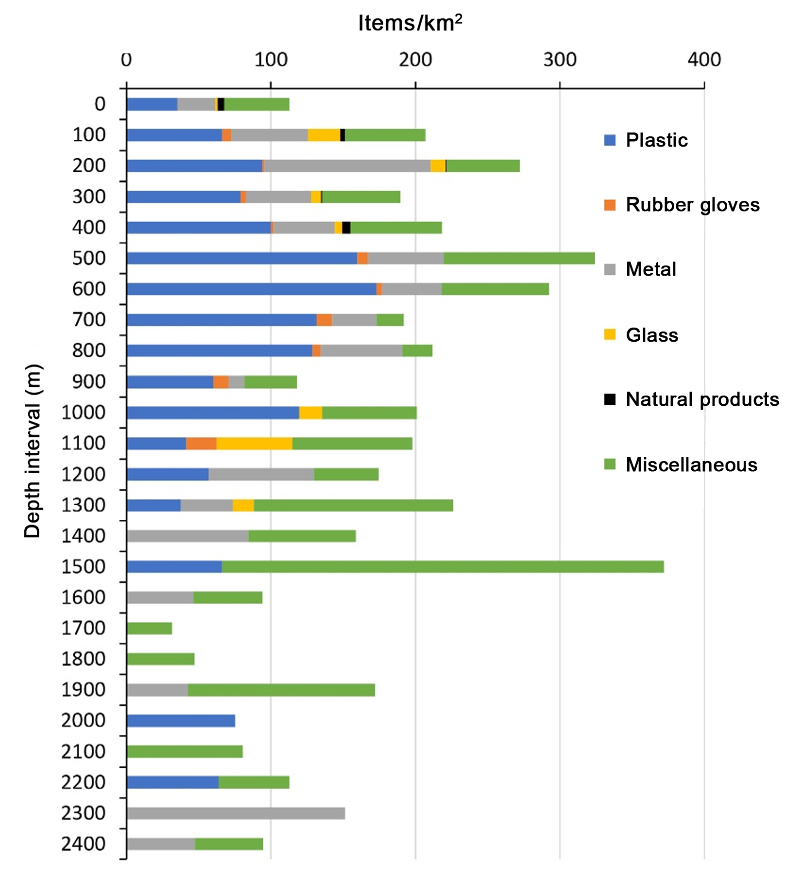
The amount and types of litter vary with depth (Figure 13). There appears to be an increase in litter density towards 600 metres. The locations with the highest litter density occur at depths shallower than approximately 700 metres. Raw data is also available via GeoNorge.
Numberoftransects
%
Totalt
3421
100
No litter
2777
81,2
With litter
644
18,8
Low density (<1000 items/km²)
409
11,9
Moderate density (1000-2000 items/km²)
172
5,0
High density (>2000 items/km²)
63
1,8
With plastic litter
303
8,9
With fishing related litter
337
9,9
Table 9. Number and percentage (%) of video transects with litter in relation to type and quantity category. Retrieved from Buhl-Mortensen et al., 2024.
Figure 13: Average number of observed items of different main categories of litter per km2 for 100-m depth intervals. Retrieved from Buhl-Mortensen et al. (2024).
The proportion of video transects with litter decreases towards the north (Table 9). The amount of litter observed is fairly similar for the northernmost areas (> 75°N) compared to areas outside Central Norway (65–70°N) (Table 10). The amount of litter decreases sharply with distance from the coast, but the trend is not as strong for fishing-related litter. The density of plastic also decreases with distance from the coast (Buhl-Mortensen et al. (2024).
Latitude (°N)
Totalnumberoftransects
Transectswithlitter
%
Ave/obs
<60
272
20
7.4
1954
60- 65
592
75
12.7
1068
65- 70
908
106
11.7
968
70- 75
920
120
13.0
635
>75
729
16
2.2
837
Table 10: Number and proportion (%) of all video transects with fishing-related litter in relation to latitude and average number of litter items for locations where litter was observed (Average/obs). Retrieved from Buhl-Mortensen et al. (2024.
4.2.3 - Plastic litter
“ Plastic was observed at 8.9% of all locations. Synthetic rope accounts for the majority (36%) of the number of observed litter items. Fishing-related plastic (fishing nets, synthetic rope, rubber gloves and other fishing-related plastic) accounts for a total of 64% of all observations of plastic litter" (Buhl-Mortensen et al., 2024) .
"The average density of plastic litter in 100-metre depth intervals increases down to around 600 metres. This increase is particularly evident in the categories of plastic film, plastic bags and other unidentified plastic. The largest amount of plastic has been observed between 400 and 1000 metres. The largest proportion of this litter comes from fisheries (synthetic rope, fishing nets and other fishing-related plastic). Fishing nets account for a large proportion of plastic litter, together with synthetic rope" (Buhl-Mortensen et al., 2024).
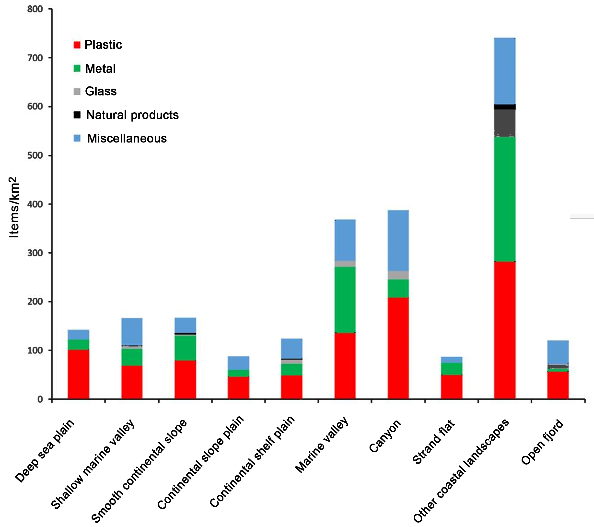
The density of litter varies with the type of marine landscape (Figure 14). It is lowest on marine plains and the continental shelf, and highest in marine valleys and gullies, as well as other coastal landscapes.
See the report ‘Plastic waste on the seabed mapped by MAREANO’ (Buhl-Mortensen et al., 2024) for more details on transects and findings.
Figure 14. Average amount of litter in different marine landscapes (landscape categories are taken from the map service at Mareano.no). Retrieved from Buhl-Mortensen et al., 2024.
4.2.4 - Geographic distribution of litter
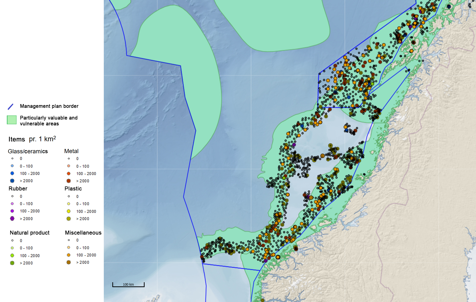
The density of different types of litter and plastic is shown in Figure 15. Detailed maps for different areas are best displayed in interactive map production site where you can zoom in on smaller areas (Mareano.no).
Figure 15. Number of litter items per km2. A: All litter categories. B: Observations of plastic litter. Retrieved from Buhl-Mortensen et al., 2024.
4.2.5 - North Sea and Skagerrak
4.2.5.1 - Mareano- observations
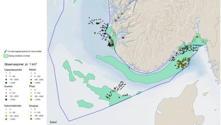
Mareano is currently mapping the North Sea, and registration of litter items is available via the mapping service at Mareano.no. In general, there is more litter in the deep inner parts of the Norwegian Trough where plastic is collected than in the coastal areas where heavier litter such as glass and metal make up the majority (Figure 16). The Norwegian Trough has been identified as a SVO, particularly due to the high density of sea pens.
Figure 16. Distribution of litter on the seabed in the North Sea recorded in the field by the mapping program Mareano (www.mareano .no). Green areas indicate particularly valuable and vulnerable areas (SVO) defined by a professional forum (Eriksen et al. 2021).
4.2.5.2 - Bycatch data from shrimp stock monitoring in the Skagerrak
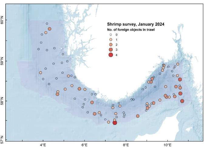
IMR records the occurrence of litter in trawl nets from the annual monitoring of shrimp populations in the Skagerrak and the Norwegian Trough in 2024 (Figure 17). At most trawl stations, litter is not found and if it is recorded, it is usually 1–3 items per trawl. Nets, nylon thread and line make up the majority of the by-catch of litter, which is therefore most likely to be fishery-related. Reported data is published in a cruise report (Søvik et al., 2024). Details of location, number and type of litter pieces are provided here.
Figure 17. The map shows the occurrence and amount of litter recorded in trawls from the shrimp stock monitoring conducted in 2024, source: Søvik et al. (2024).
4.2.6 - Norwegian Sea
4.2.6.1 - Mareano- observations
In the Norwegian Sea, Mareano has so far mainly mapped areas related to SVO areas beyond 12 nautical miles from land (Figure 18). Registration of litter items is available via the mapping service at Mareano.no. In general, there is more litter in the local depressions (troughs, channels and canyons) and in active fishing areas. Most of the litter can be linked to fishing activity.
Figure 18. Distribution of litter on the seabed in the Norwegian Sea recorded in the field by the mapping program Mareano (www.mareano .no). Green areas indicate particularly valuable and vulnerable areas (SVO) defined by "Faglig forum" (Eriksen et al. 2021).
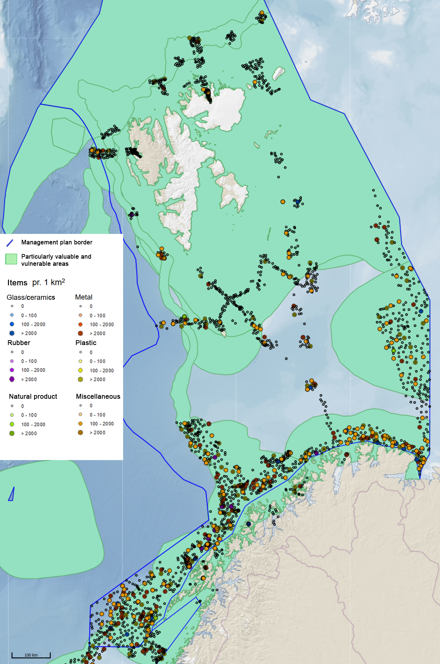
4.2.7 - Barents Sea
4.2.7.1 - MAREANO-observations
In the Barents Sea, MAREANO has mapped areas outside 12 nautical miles from mainland Norway, while in Svalbard two fjords have also been mapped (Figure 19). In general, the amount of litter is lower in the northern areas, and the highest amounts are found in local depressions (troughs, channels and canyons) and in active fishing areas. Most of the litter can be linked to fishing activity. Two areas that stand out with relatively high density are Bleiksdjupet and Hola. Bleiksdjupet is a marine canyon off Andøya, while Hola is a wide trough that crosses the continental shelf off Vesterålen.
Figure 19. Distribution of litter on the seabed in the Barents Sea recorded in the field by the mapping program MAREANO (www.mareano.no). Green areas indicate particularly valuable and vulnerable areas (SVO) defined by "Faglig forum" (Eriksen et al. 2021).
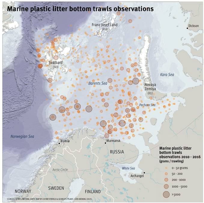
4.2.7.2 - Registration of litter in bycatch from the ecosystem surveys in the Barents Sea
Since 2010, litter has been recorded as part of the Norwegian-Russian ecosystem survey in the Barents Sea. Litter has been recorded as bycatch in bottom trawls, in pelagic trawls and as litter floating on the surface (Grøsvik et al., 2018, Eriksen et al., 2018).
The network of stations covered by the Norwegian-Russian ecosystem survey in the Barents Sea has been conducted annually since 2010, with approximately 35 nm distance between stations. Data are comparable between ships and years, since all ships use standard trawls and trawling procedures. Categories for litter records have been in relation to material types and whether they are fishery-related or not. From 2023, the protocol for the ICES Working Group on Marine Litter has been adopted by the Norwegian side (ICES 2022) (Appendix 1). Registrations of plastic in the period 2010 to 2016 are shown in Figure 20.
For the ecosystem surveys in the Barents Sea, the results are published annually in the Norwegian-Russian expedition reports, e.g. Prozorkhevich et al., 2024. Norwegian data from the expeditions can be reported to OSPAR. From 2023, the protocol from the ICES WGML was used. Corresponding data from the North Sea are reported to ICES (ICES International bottom trawl surveys). Data provide information on collection areas and sources, for example the proportion that is fishery-related.
Figure 20. Plastic as bycatch from bottom trawls from the ecosystem surveys in the Barents Sea from 2010 to 2016. Data from Grøsvik et al., 2018 .
4.3 - Sources of litter on the seabed
4.3.1 - Distribution of fisheries-related litter from the Directorate of Fisheries
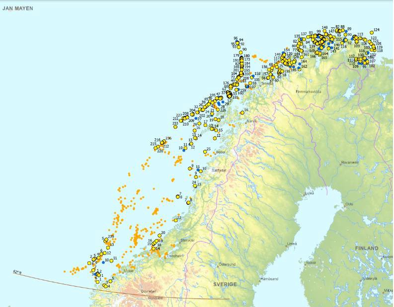
In the period 1983 – 2022, a total of approximately 25,000 nets and significant quantities of other types of gear have been recovered by the Directorate of Fisheries (Table 11, see report “Retrieval of lost fishing gear”, by Langedal & Skaar, 2023). From 2010, focus was also directed towards pots, where approximately 4,400 pots have been recovered in the last five years. Data from the Directorate of Fisheries’ clean-up expedition provides useful information about sources and accumulation sites for fishing-related litter. The cornerstone of the information base is the requirement to report lost fishing gear to the Coast Guard if the recovery is not successful. This is described in more detail in Section 69 of the Harvesting Regulations. From 2022, the option for manual reporting was removed and transferred to a solution with an electronic reporting format through Barentswatch/FiskInfo (BarentsWatch, 2015). To ensure that as many people as possible are reminded of the reporting requirement and at the same time notified of the time period for the clean-up expedition, this is announced in the relevant fisheries press at the start.
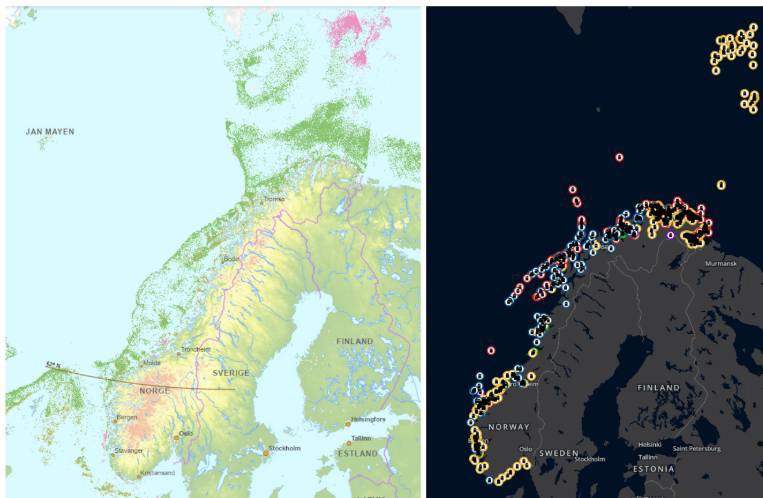
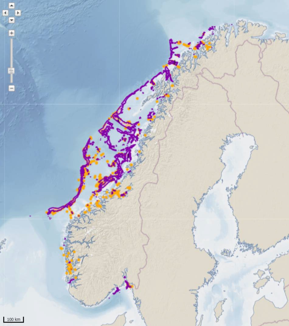
Data from the Directorate of Fisheries' clean-up expedition is mainly concentrated north of 62 degrees, where large amounts of lost fishing gear have been found (Figure 21).
Figure 21. Data from the cleanup expedition of the Directorate of Fisheries from 2017 - 2024. Yellow symbols are stations with findings. Orange symbols show the occurrence of coral reefs. Figure taken from Langedal and Skaar, 2023.
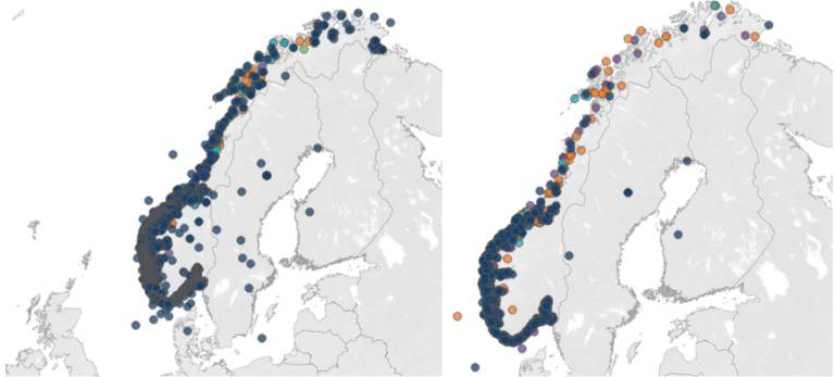
An overview taken from BarentsWatch where commercial fishermen report lost gear also shows a similar distribution of lost gear seen in clean-up operations, and when looking at national fishing activity, this also corresponds well with where lost gear is found (Figure 22).
Figure 22. Overview of fishing activity nationally (left), and overview of reported lost gear in Barentswatch (right). Data obtained from the Directorate of Fisheries through the Directorate of Fisheries' mapping solutions (Fiskeridirektoratet, 2017), and BarentsWatch (BarentsWatch, 2015).
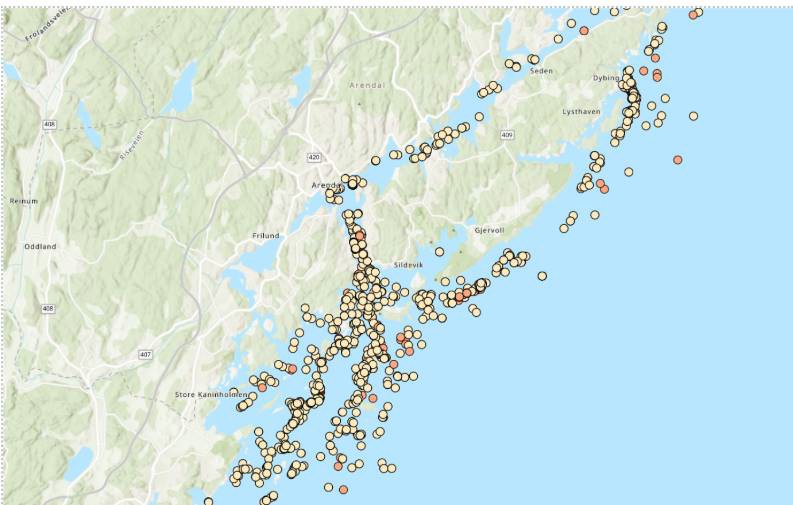
Data from reported lost fishing gear from recreational fishers along the coast and in fjords, on the other hand, show more losses of fishing gear related to recreational fishing south of Trøndelag than north of Trøndelag (Figure 23). Clean-up activities from diving clubs and other actors are also more concentrated south of Trøndelag.
Figure 23. Distribution of reported lost gear from recreational fishers from 2013-2024 (left). Distribution of reported finds of lost gear from 2013-2024 (right). Data taken from the Directorate of Fisheries' overview of lost and found gear (Directorate of Fisheries, 2017) .
Year
Nets (no)
Traps (no)
Lines (m)
Wire (m)
Ropes (m)
Trawls (m2)
Anchor/grapple (no)
Buoys/flags (no)
2019
820
1242
23700
800
56700
500
28
19
2020
681
2669
38800
4745
133800
210
66
46
2021
1000
82
78000
4700
15000
136
46
29
2022
1128
204
25200
8540
68100
125
40
39
2023
1339
229
42000
8000
30000
250
41
30
Last 5 Y
4968
4426
207700
26785
303600
1221
221
163
Table 11. Results from the last 5 years of clean-up operations in the fishing grounds along the coast. Taken from the report “Recovery of lost fishing gear/Retrieval of lost fishing gear”, by the Directorate of Fisheries (Langedal & Skaar, 2023).
4.3.2 - Ghost fishing: Lost fishing gear in coastal areas
Figure 24. Map of lost gear in and around Raet National Park outside Arendal. Source: teinevett.no (Havforskningsinstituttet, 2023). Yellow dots indicate gear retrieved before 2023, orange dots are gear retrieved in 2023 and red dots are gear retrieved in 2024.
There are currently no estimates of the total number of lost fishing gear along the Norwegian coast, but more knowledge is available in some areas. A preliminary estimate has been made for Raet National Park, indicating 10,292 (95% confidence interval: 4,749 – 18,023) ghost gear shallower than 90 meters (188 km2) (Kleiven et al., 2021). The density of gear was highest in the interval 30-60 m, compared to 0-30 m and 60 – 90 m. The calculations are based on ROV searches of randomly selected polygons in Raet National Park. The presence of ghost gear has otherwise been observed to a significant extent along the entire coast of Southern Norway. Gear recorded in the projects “Measures against ghost fishing in Raet National Park” (Kleiven et al., 2021), “Measures against ghost fishing in marine national parks” (Thorbjørnsen et al., 2023a) and “Measures against ghost fishing in Southern Norway” (ongoing project), can be seen in the map solution at teinevett.no (Figure 24) (Institute of Marine Research, 2022). You can also see an overview of lost and found gear on maps at the Directorate of Fisheries (Fiskeridirektoratet, 2017). Lost gear is mainly reported by recreational fishermen. Anyone can report found gear to the Directorate of Fisheries through the app “Fritidsfiske”, and volunteer divers from the country’s diving clubs make up a large part of those who report. Analysis of gear finds from the app between 2015 and 2020 shows that gear was recorded on 0 – 200 meters deep with an average of 22.4 m ± 14.5 m standard deviation (Thorbjørnsen et al., 2023b). The preponderance of findings in shallower water is due to the depth limitations of diving.
4.3.3 - Aquaculture
Aquaculture is also an industry that has the potential to contribute to littering. During a survey in connection with a fish farming facility, litter was observed near the facility (Figure 25). This facility is also located near a fishing-heavy town, and since the litter was not classified, it is not possible to say for sure what the source of the litter is. This study made observations of fauna and litter every 30 seconds, and can be considered an image analysis. Data are taken from an unpublished master's thesis (Vabø, 2021).
Figure 25. Distribution of litter near fish farms based on image analysis. Data taken from master's thesis (Vabø, 2021).
4.4 - Summary of litter on the seabed
4.4.1 - Accumulation areas and sources
The amount of litter in Norwegian sea areas is generally low due to horizontal transport along the seabed to greater depths due to currents, wave energy, bottom slope, etc. This leads to accumulation in certain landscape types such as fjord basins, marine canyons, troughs and channels while the amount on fish schools is low (Mareano.no). Examples of this are also seen in international research. In the central Mediterranean, most litter was found in deeper water, and most of all in marine valleys and canyons (Franceschini et al., 2019). A larger study that collected video and trawl data from European sea areas shows that the density of litter was highest in marine valleys, and that areas with high densities were mainly located closer to the coast (Pham et al., 2014).
In the open sea, industry related litter accounts for a significant proportion of registered litter on the seabed and fishing gear accounts for a large proportion. The trend is that the proportion of fisheries-related litter is increasing towards the north in Norwegian sea areas (Sources: MAREANO, Ecosysten surveys and Norwegian Directorate of Fisheries).
On the coast, litter is transported from shallow water by high wave energy and currents to deeper parts of fjords, and the amount in the intertidal zone is generally low. This means that there is little correlation between the amount of litter on the beach and the occurrence of litter on the seabed (Buhl-Mortensen & Buhl-Mortensen, 2023). The litter is most frequently found inshore, where the highest number of litter items per meter are between 50 and 100 meters (Source: mareano.no). There does not appear to be a correlation between the occurrence of litter on the beach and the amount of litter on the seabed nearby (pilot study with ROV). It must be noted that how litter is distributed from a source before it ends up on the seabed will be affected by wind and currents as well as the weight and shape of the object (Madricardo et al., 2020).
Coastal fishing is an industry that contributes a large amount of litter (Marine base map). Rivers are important sources of litter on the coast. The few available studies show that depending on weight, litter will settle on the seabed some distance out from the river mouth (pilot study with ROV in the Hardangerfjord). Locally, plastic from agriculture can make up a large part of litter transported by rivers into fjords.
4.4.2 - Conclusion
It will give an incorrect picture of the status of litter if monitoring locations are added to areas where litter is naturally removed due to ocean currents or wave energy. Furthermore, it is shown in Chapter 5 that in order to obtain good material for reliable detection of changes in litter on the seabed, monitoring should be added to locations with three or more litter items.
For the best possible monitoring, the change in litter occurrence should therefore be monitored at locations of collection/accumulation. In open ocean areas, this will be marine gullies, troughs and channels, and on the coast, the accumulation is in fjord basins, at river mouths, in areas near cities with significant fisheries or at aquaculture. Furthermore, litter easily ends up on coral reefs either due to fishing nearby or because the reef structure traps litter. It is therefore important that some such locations are included in the monitoring.
5 - Detection power of different monitoring designs
5.1 - What is statistical power ?
When analysing monitoring data, hypotheses are formulated ant the null hypothesis (H 0 ) represents no effect or change and the alternative hypothesis (H A ) an effect or change, e.g. over time.
The four possible results of a hypothesis test (Morrison, 2007; Serdar et al., 2021):
Correctly conclude that H 0 ( no c 0 hange) is true
Incorrectly conclude that H 0 (no change) is true
Correctly conclude that H A (a change) is true
Incorrectly conclude that H A (a change) is true
If one incorrectly concludes that H A is correct (4.), this is a false positive (type I error). The probability of this is represented by Alpha ( α ) and the commonly accepted error rate is 5%. This is why a statistical test is accepted as significant if the p-value is less than 0.05.
The probability of incorrectly concluding that H 0 is correct (2.) is a false negative (type II error). This is
represented by Beta ( β ). This means that a change is not detected even though it exists. For example, by taking too few samples. Statistical power is the probability of correctly concluding that a change is true (1- β ).
It is relatively common to accept a type II error rate of 20% (80% statistical power). If you want the same error rate for type I and II errors, the error rate for a type II error (β) must also be limited to 5% (95% statistical power).
The replication level required to achieve the desired statistical power depends on (1) α and β, (2) the smallest effect size one wishes to be able to measure, and (3) the distribution and variation in the underlying data. Lower tolerance for possible errors, smaller effect sizes (changes) and more variation all lead to higher requirements for data collection in order to achieve the acceptable statistical power.
Whether H A is one-sided (e.g. only wanting to detect a decline over time) or two-sided (e.g. wanting to detect either an increase or a decline ) also affects the replication requirements for achieving the desired statistical power. In a two-tailed test, the trend must be clearer in order to be detected, as the probability is divided between positive and negative changes, and the necessary replication level is therefore higher for a two-tailed test than for a one-tailed test (Serdar et al., 2021).
The probability of detecting an existing trend, and of overlooking one, are important considerations in all environmental monitoring. The aim of power analyses is to estimate the amount of data required to obtain reliable results in a monitoring programme (Morrison 2007).
5.2 - Effect size
Certain choices must be made in advance, which will affect how the power analysis is designed and which tests are performed. Central to this is what you are trying to measure. It may be a trend over time, or a change after a certain period of time; it can be specified as an increase or a decrease, and how large it must be to be of interest. This is called the effect size, and in general, a smaller change will require more accuracy and more data collection to achieve the same certainty, or statistical power, as a larger change.
The smallest change one is interested in measuring is called the minimum effect size of interest. In this case, the effect size will correspond to the smallest trend or change in waste quantities we want to investigate. We set such a threshold value because the absence of a trend (or difference between two areas) cannot be defined as precisely zero. The smaller the minimum effect size one wishes to measure, the more demanding it will be to achieve because it requires higher accuracy, for example in the form of more measurements (higher replication level).
In order for the power analyses to provide a good estimate of the amount of data that needs to be collected, it is important to use a realistic and representative distribution of the data as a basis. The more you know about the variation structure in the underlying data, the better your understanding of what needs to be collected. If there are no data from previous research or pilot tests, there is no basis for a power analysis, and it is not possible to calculate statistical power.
This means that if the study design is changed, new power analyses must be performed. It is also important to note that power analyses are only valid for the data distribution on which they are performed and the statistical test for which they were performed.
5.2.1 - Study design
In national monitoring of floating macro-litter, the aim is to be able to measure reductions of 10 and 30% over a period of five and ten years.
The basic study design used for the power analysis here is based on repeated recordings at fixed measuring stations using video transects . This allows for an analysis of the average change between intervals, such as every 5 or 10 years. Two different minimum effect sizes of interest have been investigated: a 10% and 30% change in average litter density per transect . Such a repeated design provides the greatest opportunity to detect any changes in the supply of macro-litter to the seabed. The confidence with which one can say that there has been no greater change than these effect sizes is also tested. This is important because no change in the concentration of litter on the seabed may indicate a change in supply , from some supply to no supply. See conceptual sketch, Figure 26.
Figure 26. Conceptual sketch of monitoring design. The same measuring stations are recorded at fixed intervals (e.g. every 5 years), and the average change at all locations is analysed to see if it is greater than the minimum effect size of interest (10 or 30%).
The data used for the strength analysis is from the MAREANO programme from 2006 to 2023 (described in Chapter 4). Although some video transects in this dataset are relatively long, the field of view is 3 meters. This contributes to a lower probability of encountering litter even if a transect initially passes through a littered area (Haarr et al., 2022). This is indicated by the records of 1018 pieces of litter from 3421 transects; that 81% of transects were clean, and only a few transects contained a significant number of pieces of litter (Figure 27).
Figure 27. Overview of the number of transects with different numbers of litter items observed in MAREANO 2006-2023. Note that the y-axis is log-transformed for visualisation. An increase from 1 to 2 on the y-axis therefore corresponds to x10 more transects. The number of transects are indicated above each column.
When repeatedly monitoring selected locations, these must necessarily be areas that were littered to begin with, otherwise it will not be possible to detect any decline in quantities or supply. We would like to distinguish between transects with a lot of litter and those with little, as this is useful information for the monitoring design. As there are not enough littered transects to establish clear statistically significant differences in litter density based on landscape types, depth levels or other factors, we have chosen to base our analyses on different threshold values in terms of numbers, regardless of geography or location. Different threshold values for classifying a transect as ‘heavily littered’ were therefore investigated.
Given the high proportion of clean transects, a threshold value of at least one piece of litter per transect naturally yielded the largest data set (n = 644 transects) (Table 12). A threshold value of at least four pieces of litter per transect was the highest value that provided a sufficient number of data points to fit a distribution for analysis (n = 36 transects). At a threshold of at least five pieces of litter, only 12 transects remained, and fitting a distribution was not meaningful.
The power analyses were then performed based on negative binomial distributions (suitable for describing skewed data representing the number of occurrences) fitted to a sample of transects from MAREANO with at least 1, 2, 3 or 4 pieces of litter (Table 12). Theoretical baseline data (year 0 in a monitoring programme) and data after change corresponding to the minimum effect size of interest (carried out for 10 and 30% decrease and increase on average) were then simulated based on the distributions obtained from the raw data. Random sampling of the simulated data was then performed at different replication levels and changes from the first to the second sampling period analysed using paired t-tests. It is assumed that the distribution of the differences is approximately normal given that there are over 30 location pairs and that a parametric analysis is acceptable. The procedure was repeated 1000 times for each replication level, where the starting value was 10 transects, and carried out for each level until the desired power was achieved (first 80% and then 95%). Power was calculated as the proportion of the 1000 simulations for each replication level that were significant (p < 0.05). This was done for two-tailed tests, which test the ability to measure a decline or an increase.
In addition, the same procedure was repeated where, instead of significant pairwise t-tests, it was tested whether 95% confidence intervals around the average change were within 0 ± the minimum effect size of interest (a so-called ‘equivalence test’), or, in other words, how high the replication level must be in order to achieve the desired statistical power to be able to say that the amount of litter has not changed (i.e. no new addition, which is to be considered a decrease). Being able to say with certainty that there has been no significant new addition of litter is somewhat more demanding than being able to detect whether there has been an increase (new addition) or a decrease in concentration (litter buried by sedimentation or moved out of the transects). Increasing the statistical power from 80 to 95% will require an increase in the replication level (number of locations) by 67% to measure a change and 45% to document that a change has not occurred in relation to the calculations in Table 11. The table shows that the more littered the transects being studied are (the more pieces of litter there are per transect), the fewer transects are required to detect a change with certainty. The smaller the change that can be detected (greater accuracy), the more transects are needed.
Based on this, it can be concluded that fewer transects are required to detect a large change in highly littered areas. This means that a monitoring programme based on monitoring accumulation areas will require fewer transects than one that is also based on monitoring cleaner areas (with fewer pieces of litter per transect).
Fewer transects are required to detect a change (of more than 30%, for example) than are required to rule out a similarly large change (< 30%).
There are several challenges associated with a low threshold for considering a site sufficiently littered to be suitable for monitoring litter quantities and supply. Firstly, it means that the absolute change in average litter density that constitutes a 10 or 30% change is very low (Table 11). This in turn leads to higher replication requirements in order to achieve acceptable statistical power. For example, at least 132 monitoring locations (transects) are required to detect a 30% change if a threshold value of only one item per transect is allowed at baseline (year 0), but only 47 if the threshold value is set to four items (Table 12).
Another significant challenge with a low threshold value is that it is highly vulnerable to measurement errors. Even with a spatial accuracy of ± 2 m when placing a 3 m wide transect each year, there will be a relatively high probability of missing an object that was observed during the previous registration, as well as a certain probability of discovering an object that was outside the transect last time. With low density to begin with, this represents an extremely high margin of error, especially for transects with only one object observed, where missing an object represents 100%.
This is illustrated in Figure 28, which simulates a random misregistration of either +1 or -1 object in different proportions of the transects, and then calculates the necessary replication level to achieve 80% statistical power to measure a 30% decline. This clearly shows that at a low threshold value (at least 1 piece of litter), such an error margin has a significant impact. This simulation considered both negative and positive error registrations (missing an item or finding a new one that was previously outside). If, in reality, there is a higher probability of one or the other, this will constitute a potentially large bias in the results and may lead to a type I error (false positive; concluding that a change has taken place when this was not actually the case).
Treshold* (n transect -1 )
Number of transects †
Average‡ (n transect -1 )
Average§ 10 %
Average§ 30 %
# transects needed for 80 % power
>10 %¶ change
>30 %¶ change
<10 %# change
<30 %# change
1
644
1,58
1,42
1,11
1059
132
1414
161
2
199
2,88
2,59
2,02
577
76
858
104
3
66
4,65
4,19
3,26
410
55
655
78
4
36
6,03
5,42
4,22
353
47
559
64
5
12
9,58
8,63
6,71
-
-
-
-
* Minimum litter density (number of items) in a transect to be considered a monitoring site and for the data to be included in the calculation of baseline distribution and average. †Number of transects with litter density equal to or higher than the threshold value from MAREANO 2006-2023. ‡ Average litter density in transects with the number of litter items observed equal to or higher than the thresholdvalueunderMAREANO2006-2023.§Thenewaverage(numberoflitteritemspertransect)forthedistributionof simulated data for a theoretical second sampling at a specified percentage decrease. ¶The number of transects estimated to be necessary to sample in each time period in order to achieve 80% power to detect an average change between sampling 1 and 2 ofthe specified magnitude. #The number of transects estimated to be necessary to sample in each time period in order to be able tosay with 80% certainty that there has been no change greater than the specified magnitude.
Table 12: Results of strength analysis for paired t-tests between two time periods for repeated sampling of the same transect. Note that for a threshold value of at least 5 pieces of litter per transect, there were too few data points to fit a distribution. The analyses are based on paired t-tests for two time periods (e.g. with a 5-year interval).
In order to minimise the effect of incorrect registrations due to the fact that it is not possible to place a transect on exactly the same 3 m wide path with 100% certainty every time, and to enable monitoring of changes at a lower replication level, it is recommended to set the threshold value for including a location to a minimum of three or four items of litter. Ideally, the minimum value would be even higher, but there are not enough more littered transects in the MAREANO dataset to use as a basis. If the number of litter items can be increased by increasing the transect length at each location, this is preferable, but as the probability of achieving an increased number of litter items and what the optimal transect length would be in that case cannot be calculated from the raw data due to too few findings.
Due to the extremely low number of finds per transect, it is also not possible to make calculations for different types of objects or composition. This could possibly be investigated for individual transects with unusually high density, but this would be an assessment that would have to be made on a case-by-case basis based on the data as it stands at present.
If you select transects with 3 or more pieces of litter (66 items) (Table 12), there are enough transects in the MAREANO dataset to revisit to meet the number of transects needed to detect a change of at least 30% (55 items) with 80% certainty (Figure 29). With a threshold value of at least 5 pieces of litter, there were not enough possible locations documented in MAREANO from 2006 to 2023 (Table 11) to be certain that this has not occurred. If you filter on transects with at least 4 pieces of litter to reduce the effect of false registrations, you are left with 36 pieces, which is less than the number of transects needed to detect a 30% change with the same certainty. This will therefore not be sufficient to achieve an acceptable statistical power to measure a 30% change or to be certain that this has not occurred, and even less so if the minimum effect size of interest is 10%. Additional locations must then be determined, for example from fjords and areas already surveyed in contexts other than MAREANO.
This applies even before it is considered to divide into different sea areas to investigate whether the baseline and trends differ between them. To enable this type of comparison, more data is needed to form the basis for new power analyses.
Figure 28. Required replication level to achieve 80% power to measure a 30% change simulated for different threshold values to include a location (different distributions used as a basis) and at different proportions of the transects with an error registration if the transects do not overlap exactly between years. In this case, a simulated error registration was randomly selected as +1 or -1 object. Note that if the probability of one is significantly higher than the other, this could lead to systematic misinterpretations regarding trends in litter supply and density, and not just increased uncertainty as shown here. For the distributions used as a basis, the parameters for the negative binomial distributions are adjusted to the raw data (all transects from MAREANO 2006-2023 that had a number of litter items equal to or higher than the threshold values 1, 2, 3 or 4.
Since the proportion of clean transects is high, exploratory mapping to find new suitable locations for monitoring will in any case be extensive and demanding. Such mapping must make use of all available information about where the chances are greatest of finding sufficiently littered transects for use in monitoring. One possibility is to investigate specific landscape types. Even in marine landscape types where the overall level of littering was higher, such as in marine gullies, the proportion of clean transects was still over 60%. The documented locations with 3 or more objects per transect were also spread across several different landscape types. A quarter (26%, n = 17) were in marine valleys. A fifth were on the continental shelf plain or slope. Only 6% (n = 4) were in marine gullies. In other words, it is not immediately possible to predict where sufficiently littered areas will be found based on MAREANO data. It will therefore be very cost-effective to return to already surveyed
locations from MAREANO that were sufficiently littered. This will primarily apply to monitoring at sea, as areas in fjords or harbours are not included in the MAREANO dataset. information about where the chances are greatest of finding sufficiently polluted transects for use in monitoring.
Figure 29. Location and litter density per transect where >3 items were reported in MAREANO 2006-2023. The total number of transects was 66.
Therefore, recommendations for the monitoring programme will include, as far as possible, basing monitoring at sea on repeated visits to transects already included in the MAREANO programme, where at least three pieces of litter have previously been observed, in order to avoid excessive margins of error.
Monitoring will be able to observe a 30% change since the last visit with 80% certainty, based on repeated visits to 55 MAREANO transects with at least three pieces of litter. If we assume the same distribution of litter density in each of the different sea areas, we could multiply this for each of them, but then we do not have enough existing locations in each and must search for them. It will then be important to consider whether it is easier to find more transects with as few as two litter items, accept a greater effect of misregistrations and increase the number of transects, or continue to search for more littered transects and limit the number of transects. The same applies to coastal locations.
6 - Design of monitoring programme
6.1 - Minimum solution
The Norwegian Environment Agency has outlined the following requirements for a minimum solution (start-up phase): the number of registrations is reduced to a minimum, but monitoring can be used to identify sources and accumulation areas, even though the data basis will be subject to greater uncertainty. The size of the change over time/place that can be detected as statistically significant with the minimum solution must be described.
In order to meet these requirements, it is recommended to divide the monitoring area into two: sea and coastal, as both sources and accumulation areas may differ for the coast and the sea. The number of registrations is kept as low as possible in each area, while at the same time meeting the number of registrations required to detect changes over time.
The basic study design used for monitoring here is repeated registrations at fixed measuring stations with video transects. Such a repeated design provides the greatest opportunity to detect any changes in the supply of macro-litter to the seabed, with the fewest possible measurements.
For the minimum solution, we propose a setup that should be able to detect a 30% change in accumulation areas in Norwegian sea areas and Norwegian coastal areas with 80% probability. When repeatedly monitoring selected locations, these must necessarily be areas that were littered to begin with, otherwise it will not be possible to detect any change in quantities or supply. This means that monitoring must be based on monitoring accumulation areas or ‘hotspots’ in both monitoring areas. In order to minimise the effect of incorrect recordings due to the fact that it is not possible to place a transect on exactly the same 3 m wide track with 100% certainty every time, it is recommended to set the threshold value for including a location to a minimum of three pieces of litter (Table 12).
It is recommended to repeat the transects at 5-year intervals, i.e. surveys in year 0 and year 5. For price estimates per year, see Table 13.
6.1.1 - Coast
There is currently insufficient data on a sufficiently high number of littered coastal locations to satisfy the required number of 55 transects estimated in the power analyses in Chapter 5.
Locations with sufficient density of litter must therefore be identified, and we recommend focusing the search for suitable monitoring locations based on available knowledge about accumulation areas and proximity to sources along the coast. We suggest investigating collection areas that are representative of different sources and landscape types.
Based on studies using image analysis of litter from marine base maps (Chapter 4.1) and litter from river outlets (Chapter 4.2), we can assume that there will be a higher proportion of transects with litter in data from coastal areas than in the data used for the strength analysis (based on MAREANO data). From the Marine Baseline Survey, 51 transects with observations of three or more litter items have been recorded so far, out of a total of 710 transects (Chapter 4.1).
On this background, we recommend an ambition level that corresponds to collecting locations with three or more litter items per transect (Table 13). A higher number of pieces of litter per transect will reduce the requirement for the number of transects. At least 55 transects with a density of at least three pieces of litter will be required to detect a 30% change with 80% certainty. It is necessary to take into account the need to visit several transects at the start of the project in order to have a sufisient number of transects to monitor.
If the number of transects with a higher proportion of litter (≥4 pieces of litter per transect) is identified, the requirement for the number of transects will be reduced, and new strength analyses will determine how many transects are then needed. We recommend that a new power analysis be performed after the first round of data collection to investigate whether a possible higher density of coastal litter will reduce the requirement for the number of transects, as this was not possible to estimate based on the data analysed in Chapter 5.
In order to obtain a sufficient number of transects for statistical analysis, transects should be supplemented in areas with accumulation potential. This includes fjord areas located close to densely populated areas such as cities or towns, close to ports, coastal marine valleys, fjord areas near sources, and areas close to river outlets. In order to maximise the probability of detecting a higher number of pieces of litter per location, it is recommended to consider using longer transects.
For price estimates for the coast, please refer to Table 4. We assume that the number of transects that can be surveyed varies between 10 and 15 per day (12-hour shift) depending on transport time and distance between stations.
6.1.2 - Ocean
In order to detect possible changes in accumulation areas at sea, we propose that all three management plan areas be merged into one marine area and that transects in the Mareano database with three or more litter items per transect be revisited at the same position as before. This will eliminate the need to search for new accumulation areas at sea, which will result in significant savings.
If the transects are repeated at 5-year intervals, i.e. surveys in year 0 and year 5, it will also be possible to provide answers regarding changes over time for registrations in year 0, since the transects have already been visited in the MAREANO programme.
For the price estimate for the sea, we estimate 10–12 transects per day, depending on depth, transport time and distance between stations. We refer to the cost estimate in Table 4.
Total number of transects to be revisited for the minimum solution: At least 55 for both coastal areas and open sea areas where the three management plan areas are surveyed together, a total of at least 110 transects.
6.2 - Intermediate solution
As an intermediate solution, we propose building on the minimum solution, which would only include priority areas with high accumulation potential. In addition, we propose that vulnerable natural areas be included. The number of stations will still be kept at a level where there is an 80% probability of detecting a 30% change in coastal areas and marine areas, respectively.
When it comes to vulnerable habitats, the type of litter will be decisive for the potential damage. For example, ghost fishing can be very destructive to vulnerable species in an area, and the presence of gear (pots, nets, etc.) that contributes to this is important to monitor.
A scaled-down monitoring strategy in such areas could therefore be based on the presence/absence of lost fishing gear such as nets or pots in a transect or area. Strength calculations will have to be made based on the first round of data collected to determine the number of transects required. For price estimates, see Table 13.
Proposal for vulnerable areas
Areas with a high density of vulnerable species, e.g. coral reefs, coral forests, sea pen communities, seagrass beds and sponge areas (Figure 30). Such vulnerable habitats, especially coral reefs, have a complex spatial structure which, in addition to being a habitat for a multitude of other species, also acts as a ‘trap’ for litter. It is common to find lost fishing equipment (lines and nets) on coral reefs.
In this report, we propose several areas with coral reefs in coastal areas that could be suitable for monitoring seabed litter. From north to south: Stjernsund, Bleiksdjupet, Hola, Breisunddjupet, Breisundet, Langenuen, Midtsundet, and Hvaler National Park. Bleiksdjupet is a deep marine ravine with occurrences of hard bottom coral forests. This area also represents the ‘deep sea’ with depths of up to 1500 m. In the North Sea and Skagerrak, the deep parts of the Norwegian Trench are a collection area for plastic waste and also have large densities of seaweed of several species.
Figure 30. Example of vulnerable areas such as coral reefs in Norwegian sea areas. Orange circles: Observed coral reefs. Purple areas: Areas modelled as having the potential for coral reefs. Source: Mareano.no
6.3 - Full-Scale program
A full-scale monitoring programme should provide detailed information on the quantities and types of litter on the seabed at regional level, for different water types or coastal sections (minimum for the Skagerrak/North Sea, Norwegian Sea and Barents Sea regions).
In order to be able to detect a 30% change in each of the North Sea/Skagerrak, Norwegian Sea and Barents Sea management plan areas with 80% probability, for sea areas and coastal areas separately, repeated visits to a sufficient number of stations with a sufficient amount of litter (≥ 3 pieces of litter) in each area (a total of 55 transects per area) are recommended. Transects with three or more litter items have been selected to reduce uncertainty associated with possible misregistration of litter in a video transect with a width of 3 m, as shown in Figure 28 (Chapter 5). We recommend a survey interval of 5 years (year 0 and year 5).
As of today, there are not enough known locations with sufficient amounts of litter in each of the sea areas (North Sea/Skagerrak, Norwegian Sea, Barents Sea) in the MAREANO dataset to satisfy the required number of transects. It is recommended to start with the already known locations in each sea area that meet the requirements, and supplement with additional stations through focused searches in areas with a high probability of litter accumulation. These must be based on available knowledge about sources and marine landscape types with a higher proportion of littered transects based on previous surveys (such as marine ridges and marine valleys). In the MAREANO data, the documented locations with three or more objects per transect were spread across several different landscape types, but a quarter (26%, n = 17) were in marine valleys. A fifth were on the continental shelf plain or slope. About 6% (n = 4) were in marine gullies. For the North Sea/Skagerrak, the Norwegian Trench has been identified as a collection area for litter, while litter is more easily transported further along the continental shelf.
Along the coast, it is recommended to locate a sufficient number of sites in a full-scale setup in order to detect a 30% change with 80% probability. In coastal areas, the types of sources and supply rates may vary between regions, and it is recommended that a full-scale solution take this into account by dividing the coast into regions where a sufficient number of transects or locations are planned in each region. It is recommended that the regions correspond to the coastline along the Skagerrak, North Sea, Norwegian Sea and Barents Sea.
The total number of transects to be revisited in a full-scale setup is 55 x 3 (sea) + 55 x 3 (coast), where each transect contains ≥3 pieces of litter. The number of transects can be adjusted downwards if a high proportion of transects with higher density are found (47 transects with ≥4 pieces of litter, etc.). See Chapter 5, Table 12 for details. For price estimates, see Table 13.
6.3.1 - Proposed areas
Coast
Færder: Areas with a lot of lost fishing gear. Areas of particular interest may be near small boat harbours and the bottom of underwater slopes, where lost fishing gear tends to accumulate.
River outlets: Drammenselva and Glomma River are the largest rivers that flow into the Inner Skagerrak on the Norwegian side. A report on marine plastic in Skagerrak showed, that a measuring station outside the mouth of the Drammenselva had some of the highest findings of microplastics (Albretsen et al., 2018).
Coastal areas as shown in marine base maps, section 4.1.
Breisundet: Area with high densities of lost fishing gear. Also an area with highly vulnerable natural features, such as coral reefs.
Nordth Sea/Skagerrak
The Norwegian Trench has been shown to be a type of marine landscape (marine valley) where higher densities of seabed litter have been observed, but in the case of the Skagerrak, the Norwegian Trench also includes areas where ships and ammunition were dumped after World War II. Mareano has found that the deepest part of the Norwegian Trench acts as a collection point for plastic. This may be related to current conditions, where short- or long-distance transported plastic film sinks to the bottom. Closer to the coast, Mareano has found less plastic, and the litter consists of heavier materials (mainly glass and metal).
Norwegian Sea
Breisunddjupet is located just outside the 12-mile limit in the extension of Breisundet.
The area can be characterised as a marine valley and has an area with elongated coral reefs that are protected from bottom trawling. Mareano has mapped six locations in the deep trench itself and several locations in the surrounding area.
Barents Sea
Marine troughs and canyons examples.
Bleiksdjupet (off Andøya) is a canyon where Mareano has mapped the seabed and found accumulations of litter. This area covers depths from approx. 300 to over 1000 m, and may be a good candidate to represent the deep sea.
Hola (Vesterålen) is a trough that crosses the continental shelf and has a high density of elongated coral reefs.
Level
Numbertransect
Time(days
Total cost (1000 NOK)
Comments
Minimumsolution
Ocean
55
5 + travel
5 212
20 transect (2 days) depth 200-300 m, 15 transect (1 day) depth 300-400 m, 20 transekt (2 days) depth 400-600 m.
Coast
55
5 + travel
833
15 transect depth 20-100 m (1,5 day), 15 transect depth 100-200 m (1,5 day), 25 transect depth 200-500 m (2 days).
Total
110
10 + travel
6 045
Intermediate solut.
Vulnerable ecosystems: In addition to minimum solution
55
5 + travel
1 402
Coast: 10 transect depth 20-200 m (1 day), 15 transect depth 200-500 m (1 day). Ocean: 15 transect (1 day) depth 200-300 m, 15 transect (2 days) depth 300-500 m.
Total
165
15 + travel
7 447
Full-scaleprogr.
Ocean
165
17 + travel
8 044
60 transect (4 days) depth 200-300 m, 45 transect (3 days) depth 300-400 m, 60 transect (4 days) depth 400-600 m.
Coast
165
14 + travel
1 374
55 transect depth 20 - 100 m (4 days), 55 transect depth 100-200 m (4 days), 55 transect depth 200-500 m (3 days).
Vulnerable ecosystems
55
5+ travel
1 402
Same as in intermediate solution
Totalt
385
36 + travel
10 820
Table 13: The calculation is based on Table 4, where the transects per day are close to each other. For the sea, a daily rate of NOK 400,000 per day for seagoing vessels has been used as a basis. In the first year, a greater effort must be expected as transects with ≥3 pieces of litter must be identified. Reporting costs must be added to the total amount. Travel costs between the four locations must be added.
7 - References
Albretsen J, Huserbråten M, Mathisen HL og Naustvoll L-J, 2018. Marin plast i Skagerrak. Rapport fra Havforskningen Nr 38-2018. ISSN: 1893-4536. Pp 25.
Bajaj R, Garg S, Kulkarni N, Raut R. 2021. Sea Debris Detection Using Deep Learning : Diving Deep into the Sea. In: 2021 IEEE 4 th International Conference on Computing, Power and Communication Technologies, GUCON 2021. Institute of Electrical and Electronics Engineers Inc.
Bancud GE, Labanon AJ, Abreo NA, Kobayashi V. 2023. Combining Image Enhancement Techniques and Deep Learning for Shallow Water Benthic Marine Litter Detection. In: Koprinska I, Mignone P, Guidotti R, Jaroszewicz S, Fröning H, Gullo F, et al., editors. Machine Learning and Principles and Practice of Knowledge Discovery in Databases ECML PKDD 2022 Communications in Computer and Information Science [Internet]. Springer Nature Switzerland. (Communications in Computer and Information Science; vol. 1752). Available from: https://link.springer.com/10.1007/978-3-031-23618-1
Buhl-Mortensen L, Buhl-Mortensen P. 2023. Søppelforekomster på havbunn i kyst: Et pilot-prosjekt. Rapport fra havforskningen, 2022-49, ISSN:1893-4536
Buhl-Mortensen P, Buhl-Mortensen L. 2014. Diverse and vulnerable deep-water biotopes in the Hardangerfjord. – Marine Biology Research 10: 253-267, http://dx.doi.org/10.1080/17451000.2013.810759
Buhl-Mortensen P, Buhl-Mortensen L, 2018. Impacts of Bottom Trawling and Litter on the Seabed in Norwegian Waters. Front. Mar. Sci. 5 :42. Doi :10.3389/fmars.2018.00042
Cau A, Sbrana A, Franceschini S, Fiorentino F, Follesa MC, Galgani F, et al. 2024. What, where, and when: Spatial-temporal distribution of macro-litter on the seafloor of the western and central Mediterranean sea. Environmental Pollution. 342. https://doi.org/10.1016/j.envpol.2023.123028
Chen X, Lu Y, Wu Z, Yu J, Wen L. 2020. Reveal of Domain Effect: How Visual Restoration Contributes to Object Detection in Aquatic Scenes.: http://arxiv.org/abs/2003.01913
Chin CS, Bo Hui Neo A, See S. 2022. Visual Marine Debris Detection using Yolov5s for Autonomous Underwater Vehicle. In: Proceedings - 2022 IEEE/ACIS 22nd International Conference on Computer and Information Science, ICIS 2022. Institute of Electrical and Electronics Engineers Inc.; 2022. p. 20–4.
Deng H, Ergu D, Liu F, Ma B, Cai Y. An embeddable algorithm for automatic garbage detection based on complex marine environment. Sensors. 2021 Oct 1;21(19).
Đuraš A, Wolf BJ, Ilioudi A, Palunko I, De Schutter B. A Dataset for Detection and Segmentation of Underwater Marine Debris in Shallow Waters. Sci Data. 2024 Dec 1;11(1).
Eriksen et al. 2021. Særlig verdifulle og sårbare områder (SVO) i norske havområder - Miljøverdi En gjennomgang av miljøverdier og grenser i eksisterende SVO og forslag til nye områder. Rapport fra havforskningen 2021-26, 308p.
Fleet D, Vlachogianni T, Hanke G. 2021. Joint list of litter categories for marine macro-litter monitoring [Internet]. Publications Office of the European Union; 2021 [cited 2024 Oct 15]. Available from: doi:10.2760/127473
Franceschini S, Mattei F, D’Andrea L, Di Nardi A, Fiorentino F, Garofalo G, et al., 2019. Rummaging through the bin: Modelling marine litter distribution using Artificial Neural Networks. Mar Pollut Bull. 149:110580. https://doi.org/10.1016/j.marpolbul.2019.110580
Galgani F, Giorgetti A, Le Moigne M, Brosich A, Vinci M, Lipizer M, et al., 2022. EMODnet Thematic Lot n°4-Chemistry Guidelines and forms for gathering marine litter data: beach and seafloor trawlings. Version 7.1 [Cited 2024 Oct 15]. Available from: https://doi.org/10.6092/15c0d34c-a01a-4091-91ac-7c4f561ab508
Grøsvik BE, Prokhorova T, Eriksen E, Krivosheya P, Horneland PA, Prozorkevich D. 2018. Assessment of marine litter in the Barents Sea, a part of the joint Norwegian-Russian ecosystem survey. Front. Mar. Sci., 06 March 2018 | https://doi.org/10.3389/fmars.2018.00072
Haarr, M.L., Falk-Andersson, J., Fabres, J., 2022. Global marine litter research 2015–2020: Geographical and methodological trends. Science of The Total Environment 820, 153162. https://doi.org/10.1016/j.scitotenv.2022.153162
Havforskningsinstituttet, 2022. Tema: Tips for godt teinevett. [Internett] (Oppdatert 03.12.24). Tilgjengelig på: teinevett.no . Besøkt 18.11.24.
Hong J, Fulton M, Sattar J. 2020. TrashCan: A Semantically-Segmented Dataset towards Visual Detection of Marine Debris. 2020 Jul 16; Available from: http://arxiv.org/abs/2007.08097
ICES. 2022. ICES manual for seafloor litter data collection and reporting from demersal trawl samples. ICES Techniques in Marine Environmental Sciences Vol. 67. 16 pp. https://doi.org//10.17895/ices.pub.21435771
Jalil B, Maggiani L, Valcarenghi L. 2023. Comparative analysis of machine learning algorithms for the classification of underwater marine debris. In: 2023 IEEE International Workshop on Metrology for the Sea; Learning to Measure Sea Health Parameters, MetroSea 2023 - Proceedings. Institute of Electrical and Electronics Engineers Inc. Pp. 116– 20.
Kleiven AR, Thorbjørnsen SH, Aslaksen T, 2021. Tiltak mot spøkelsesfiske i Raet Nasjonalpark - Arbeidsrapport. Rapport fra Havforskningen. Arendal: Havforskningsinstituttet.
Langedal G og Skaar KL. 2024. Opprensking av tapte fiskeredskaper/Retrieval of lost fishing gear, rapport fra Fiskeridirektoratet.
Madricardo F, Ghezzo M, Nesto N, Mc Kiver WJ, Faussone GC, Fiorin R, Riccato F, Mackelworth PC, Basta J, De Pascalis F, Kruss A, Petrizzo A and Moschino V (2020) How to Deal With Seafloor Marine Litter: An Overview of the State-of-the-Art and Future Perspectives. Front. Mar. Sci. 7:505134. doi: 10.3389/fmars.2020.505134
MSFD Technical Group on Marine Litter. MSFD Technical Group on Marine Litter. Guidance on the Monitoring of Marine Litter in European Seas An update to improve the harmonised monitoring of marine litter under the Marine Strategy Framework Directive. In 2023 [cited 2024 Oct 15]. https://doi.org/10.2760/59137
Morrison, L.W., 2007. Assessing the Reliability of Ecological Monitoring Data: Power Analysis and Alternative Approaches. Natural Areas Journal 27, 83–91. https://doi.org/10.3375/0885- 8608(2007)27[83:ATROEM]2.0.CO;2
NORCE. 2020. Velle G, Barlaup B, Espedal EO, Haave M, Landro Y, Normann E, Postler C, Skoglund H, Stranzl S, Stöger E og Wiers T, Plast i elver på Vestland. LFI rapport nr. 390 2020.
Pham CK, Ramirez-Llodra E, Alt CHS, Amaro T, Bergmann M, et al. 2014. Marine litter distribution and density in European seas, from the shelves to deep basins. PLoS One 9 (4), e95839. http://dx.doi.org/10.1371/journal.pone.0095839 .
Politikos D V., Adamopoulou A, Petasis G, Galgani F. 2023. Using artificial intelligence to support marine macrolitter research: A content analysis and an online database. Vol. 233, Ocean and Coastal Management. Vol 233 15 February 2023, 106466. https://doi.org/10.1016/j.ocecoaman.2022.106466
Politikos D V., Fakiris E, Davvetas A, Klampanos IA, Papatheodorou G. 2021. Automatic detection of seafloor marine litter using towed camera images and deep learning. Mar Pollut Bull. Vol 164, 111974. https://doi.org/10.1016/j.marpolbul.2021.111974
Singh, N., Bhat, A. A systematic review of the methodologies for the processing and enhancement of the
Serdar CC, Cihan M, Yücel D, Serdar MA. 2021. Sample size, power and effect size revisited: simplified and practical approaches in pre-clinical, clinical and laboratory studies. Biochemia Medica vol. 31, Issue 1. https://doi.org/10.11613/BM.2021.010502
Søvik G, Zimmermann F, Olsen SAa, Thangstad TH. 2024. Toktrapport: Overvåkning av rekebestanden i Sør-Norge. Havforsningsinstituttet: Bergen.
Thorbjørnsen SH, Kleiven AR, Aslaksen T, Jørgensen T, Kerlefsen KV, Loga SR og Numme SS, 2023a. Tiltak mot spøkelsesfiske i marine nasjonalparker - Arbeidsrapport. Rapport fra Havforskningen. Arendal: Havforskningsinstituttet.
Thorbjørnsen SH, Synnes AEW, Løset ID, Kleiven AR, 2023b. Hazard and catch composition of ghost fishing gear revealed by a citizen science clean-up initiative. Marine Policy 148, 105431. https://doi.org/10.1016/j.marpol.2022.105431
Vabø, Ø. S. (2021). Distribution, diversity, and environmental drivers of benthic megafaunal communities in five
western Norwegian fjords. Mastergradsoppgave, Universitetet i Bergen, Havforskningsinstituttet.
Xue B, Huang B, Wei W, Chen G, Li H, Zhao N, et al. An Efficient Deep-Sea Debris Detection Method Using Deep Neural Networks. IEEE J Sel Top Appl Earth Obs Remote Sens. 2021;14:12348–60.
8 - Appendix 1. Litter categories for recording bycatch in trawls.
Categories of litter (A-F) with respective subcategories for waste type (ICES, 2022) for recording bycatch in trawls.
Material-type
Code
Norwegian name on litter types
Norwegian explanation
English name on litter types
English description
A Plastic (Plast)
A 1
Flaske
Beholder med smal hals.
Bottle
Container with a narrow neck.
A 2
Flak
Myk plastfolie, inkludert innpakningsmateriale.
Plate
Soft plastic foil, including wrapping material.
A 3
Pose
Alle typer poser laget av plast, inkludert nettingposer.
Bag
All types of bags made of plastic, including mesh bags.
A 4
Lokk og skrukork
Alle typer korker/lokk (f.eks. flaskekorker, sportshetter og pennelokk).
Cap and lids
All types of caps/lids (e.g. bottle caps, sports caps, and pen lids).
A 5
Fiskeline (monifilament)
Én enkelt plastline, ikke nødvendigvis fiskerelatert.
Fishing line (monofilament)
One single strain of plastic, not necessarily fishing related.
A 6
Fiskeline (flere sammenbundet)
Flere enkeltliner av plast, viklet sammen.
Fishing line (entangled)
Multiple single strains of plastic, entangled together.
A 7
Tau (av syntetiske fibre)
Tvinnede filamenter laget av syntetiske fibre.
Synthetic rope
Twined filaments made of synthetic fibres.
A 8
Fiskegarn
Laget av syntetiske fibre vevd inn i en gitterlignende struktur.
Fishing net
Made from synthetic fibres woven into a grid-like structure.
A 9
Kabelbindere
En tynn plastremse med riller på den ene kanten for å tillate en stramme- og låsemekanisme. Også kjent som buntebånd, strips eller slangebånd.
Cable ties
A thin strip of plastic with ridges on one edge to allow for a tightening and locking mechanism. Also known as zip ties or hose ties.
A 10
Stroppebånd
Syntetisk vevd stripe som brukes til å sikre emballasje.
Strapping band
Synthetic woven strip used to secure packaging.
A 11
Kasser og beholdere
Fra små oppbevaringsbokser, beholdere, kasser, brett og andre lagringsprodukter eller emballasje for mat og andre forbruksvarer, til større produkter som stablekasser, smådeleskuffer og lagertanker, inkludert industrikasser (f.eks. fiskekasser). Også plastkopper.
Crates and containers
From small plastic storage boxes, containers, crates, trays, and other storage products or packaging for food and other consumer goods, to larger products such as stack/nest boxes, small parts bins, and storage tanks, including industrial crates (e.g. fish boxes). Also plastic cups.
A 12
Bleier
En type engangsundertøy, mest brukt til spedbarn, men kan komme i voksenstørrelser.
Diapers
A type of single use underwear, most commonly used for infants, but can come in adult sizes. Also known as nappies.
A 13
Sanitetshåndklær og tamponger
Inkluderer tamponger, applikatorer og truseinnlegg med tilhøende plaststrimler.
Sanitary towels and tampons
Includes tampon applicators, panty liners, and their plastic strips.
A 14
Annet
Ugjenkjennelige gjenstander og gjenstander som ikke passer inn i andre kategorier, inkludert harde plastbiter.
Other
Unrecognisable items and items not fitting in other categories, including hard plastic pieces.
A 15
Munnbind
Medisinske engangsmasker, FFP2, FFP3 og ansiktsskjermer.
Medical mask
Single use medical masks, FFP2, FFP3, and face shields.
A16
Annen fiskerirelatert plast
Plastartikler knyttet til fiske- og akvakulturaktiviteter (f.eks. teiner, ruser og feller). Denne kategorien inkluderer ikke fiskegarn som dekkes av kategori A8.
Other fishing related plastics
Plastic items related to fishing and aquaculture activities (e.g. pots and traps). This category does not include fishing nets which are covered in category A8.
B Metal (Metall)
B 1
Bokser (mat)
Metallbokser, uavhengig av form, brukes til matoppbevaring.
Cans (food)
Metal cans, independent of shape, used for food storage.
B 2
Bokser (drikke)
Metallbokser, uavhengig av form, brukt til drikkevarer. For væsker som ikke er beregnet på konsum, bruk kategori B4.
Cans (beverage)
Metal cans, independent of shape, used for beverages. For liquids not meant for human consumption, use category B4.
B 3
Fiskerirelatert
Metallgjenstander relatert til fiskeaktiviteter, som linefiske og/eller tråling (f.eks. kroker, sjakler, kjetting og søkke).
Fishing related
Metal items related to fishing activities, such as line fishing and/or trawling (e.g. hooks, shackles, ticklers, and sinkers).
B 4
Beholder/spann
Sylindriske eller avlange beholdere og spann (f.eks. for olje eller maling).
Drums
Cylindrical or oblong containers and pots (e.g. for oil or paint).
B 5
Elektrisk eller mekanisk utstyr (hvitevarer)
Elektriske eller mekaniske enheter.
Appliances
Electric or mechanical devices.
B 6
Bildeler
Alle bilrelaterte deler som hovedsakelig består av metall.
Car parts
All car related items which mainly consist of metal.
B 7
Kabler
Metallkabler og elektriske ledninger.
Cables
Metal cables and electrical wires.
B 8
Annet
Ugjenkjennelige gjenstander eller gjenstander som ikke passer i andre kategorier, inkludert metallbiter og skruer.
Other
Unrecognisable items or items that do not fit in other categories, including metal pieces and screws.
C Rubber (Gummi)
C 1
Støvler, fottøy
En støvel laget av gummi.
Boots, footwear
A boot made of rubber.
C 2
Ballonger
Tynn oppblåsbar gjenstand av gummi (f.eks. brukt som leketøy eller dekorasjon).
Ballons
Thin rubber inflatable object (e.g. used as a toy or decoration).
C 3
Trålspoler
En del av trålutstyret (runde eller rørformede gjenstander forbundet med tråd, wire eller garn for å rulle over havbunnen). Også kjent som rockhoppere.
Bobbins (fishing) (rockhoppers)
Part of the fishing net (a round or tube-shaped object connected by thread, wire, or net to roll over the seafloor). Also known as rockhoppers.
C 4
Dekk
Tykk gummiring som monteres rundt ytterkanten av et kjøretøyhjul.
Tyre
Thick rubber ring that is fitted around the outer edge of a vehicle wheel.
C 5
Hanske
Klær som bæres på hender og håndledd laget av kunstig eller naturlig gummi (f.eks. hansker brukt i fiskeri og laboratoriehansker av nitrilgummi).
Glove
Piece of clothing that is worn on the hands and wrists made from artificial or natural rubber (e.g. gloves used in fisheries and nitrile rubber laboratory gloves).
C 6
Annet
Ugjenkjennelige gjenstander og gjenstander som ikke passer i noen andre gummikategorier ovenfor.
Other
Unrecognisable items and items that do not fit in any other rubber categories above.
D Glass and ceramics (Glass og keramikk)
D 1
Krukke
En beholder med bred munn laget av glass eller keramikk.
Jar
A wide-mouthed container made of glass or pottery.
D 2
Flaske
En glassbeholder med smal hals.
Bottle
A glass container with a narrow neck.
D 3
Bruddstykke
Fragment av en større gjenstand laget av glass eller keramikk.
Piece
Fragment of a larger item made of glass or ceramics.
D 4
Annet
Ugjenkjennelige gjenstander og gjenstander som ikke passer inn i andre kategorier (f.eks. drikkeglass, kopper, keramiske fliser eller murstein).
Other
Unrecognisable items and items that do not fit in other categories (e.g. drinking glasses, cups, ceramic tiles, or bricks).
E Natural products (Naturprodukter)
E 1
Prosessert tre
Bearbeidede gjenstander laget av tre (f.eks. kosteskaft, planker eller rigg).
Wood processed
Processed objects made of wood (e.g. broomstick, planks, or rigging).
E 2
Tau
Tau laget av naturlige fibre, som bomull, sisal, hamp eller kokosfibre. For tau laget av syntetiske fibre, se kategori A7.
Rope
Ropes made from natural fibres, such as cotton, sisal, hemp, or coir. For ropes made from synthetic fibres see category A7.
E 3
Papir og papp
For eksempel aviser eller kraftige papirbaserte produkter.
Paper and cardboard
For example, newspapers or heavy-duty paper-based products.
E 4
Palle
Flat transportstruktur i tre.
Pallets
Flat wooden transport structure.
E 5
Annet
Ugjenkjennelige, menneskeskapte, bearbeidede gjenstander og gjenstander som ikke passer inn i andre kategorier, for eksempel skifertakstein, brostein, betong, slaggstein eller kull. Når kildematerialet er et naturprodukt som med hensikt har blitt varmet opp for å produsere et menneskeskapt materiale, tilhører det kategori D (f.eks. murstein eller ting laget av glass).
Other
Unrecognisable, man-made, processed items and items that do not fit in other categories, such as slate roof tiles, cobbles, concrete, cinder stone, or coal. When the source material is a natural product that has been intentionally heated to produce a man-made material, it belongs to category D (e.g. bricks or things made of glass).
F Miscallaneous (Diverse)
F 1
Klær og filler
Alle typer klær, tekstil og vevde produkter, bortsett fra gummihansker som tilhører underkategori C5.
Clothing and rags
All types of clothing, textile and woven products, except for rubber gloves which belong to subcategory C5.
F 2
Sko
Alle typer fottøy, bortsett fra gummistøvler som tilhører underkategori C1.
Shoes
All types of footwear, except for rubber boots which belong to subcategory C1.
F 3
Annet
Ugjenkjennelige gjenstander og gjenstander som ikke passer inn i andre kategorier.
Other
Unrecognisable items and items that do not fit in other categories.