Northern shrimp (Pandalus borealis) in the Barents Sea (ICES Subareas 1 and 2), including the Svalbard fishery protection zone (FPZ) and coastal shrimp along the Norwegian coast north of 62°N, is defined as one stock. Norwegian and Russian vessels exploit the stock in the entire area, while vessels from other nations are restricted to the Svalbard FPZ and the “loophole” area.
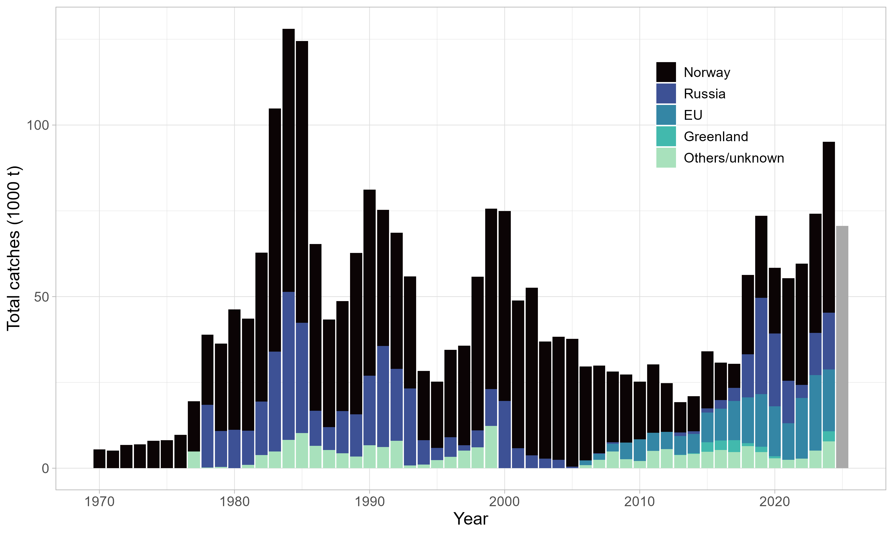
Norwegian vessels initiated the fishery in 1970. As the fishery developed, vessels from several nations joined and landings increased rapidly (Figure 1). Vessels from Norway, Russia, Iceland, Greenland, Faroe Islands, United Kingdom and the EU have participated in this fishery on a regular basis. There is no overall management plan or total allowable catch (TAC) established for this stock, but a separate TAC has been set for the Russian Exclusive Economic Zone (EEZ). In the Norwegian EEZ and Svalbard FPZ, the fishery is only regulated through effort control. Licenses are required for the Russian and Norwegian vessels. In the Norwegian EEZ and Svalbard FPZ, the fishing activity of these license holders is constrained only by bycatch regulations, whereas the activity of third country fleets operating in the Svalbard FPZ is also restricted by the number of effective fishing days and the number of vessels by country. The minimum legal stretched mesh size in the trawl is 35 mm. Bycatch is minimized by mandatory sorting grids and by the temporary closing of areas where excessive bycatch of juvenile cod, haddock, Greenland halibut, redfish or shrimp <15 mm carapace length (CL) is registered.
1.1 - Landings
Landings have increased from a lowpoint of 19 248 t in 2013 to an average of 68 533 t in the past 5 years (Figure 1). Preliminary information for 2025 indicate total landings in line with 2023 and therefore a decrease after the peak in 2024. Total catches in the fishery are assumed to be equivalent to reported landings.
2015
2016
2017
2018
2019
2020
2021
2022
2023
2024
20251
Norway
16 618
10 898
7 010
23 126
23 924
19 115
29 890
35 290
34 782
49 799
34 254
Russia
1 151
2 491
3 849
12 561
28 081
21 265
12 379
3 809
12 288
16 570
10 889
Others
16 252
17 359
19 582
20 653
21 576
17 999
13 085
20 481
27 114
28 794
25 463
Tota
34 022
30 748
30 441
56 341
73 582
58 380
55 354
59 580
74 184
95 163
70 606
1 Preliminary
Table 1: Recent reported landings in tonnes, as used for the assessment by fleet. Others include EU, Greenland, Iceland, Faroes and United Kingdom. Landings for 2025 are predicted based on preliminary reporting.
Figure 1: Total catches by country and year. Catches are assumed to be identical to reported landings. Value for 2025 is predicted based on preliminary reporting.
1.2 - Discards and bycatch
Discards of shrimp cannot be quantified but are assumed to be small as the fishery is not limited by quotas. Bycatch rates of other species are estimated from at-sea inspections and research surveys and are corrected for differences in gear selection pattern, and raised with the corresponding shrimp catches from logbooks to give an overall bycatch estimate (Breivik et al., 2017). Revised and updated discards estimates (1983–2017) of cod, haddock and redfish juveniles in the Norwegian commercial shrimp fishery in the Barents Sea were available in 2018. Since the introduction of the Nordmøre sorting grid in 1992, only small individuals of cod, haddock, Greenland halibut, and redfish, in the 5–25 cm size range, are caught as bycatch. Collecting bags, an extra codend mounted on the shrimp trawl for catching ground fish as bycatch, are being used by some EU vessels (ICES, 2022a).
1.3 - Ecosystem considerations
Since the 1980s, the Barents Sea has shifted from a situation with high fishing pressure, cold conditions and low demersal fish stock levels, to a state of high levels of demersal fish stocks, reduced fishing pressure and warmer conditions. A substantial decline of Atlantic cod (Gadus morhua) over the past years may, however, confirm a trend reversal. Cod is a major predator of northern shrimp, but there is no clear evidence of predation as driver of shrimp population dynamics. More detailed information on ecosystem dynamics in the Barents Sea are provided in reports of the ICES Working Group on the Integrated Assessment of the Barents Sea (ICES, 2022b) and the Barents Sea ecosystem survey (Prozorkevich et al., 2024).
2 - Input data
2.1 - Commercial fishery data
Information on catches by country were retrieved from the ICES database and complemented with catch information from the Norwegian landings register for the assessment year. Logbook data are normally available only from the Norwegian fleet.
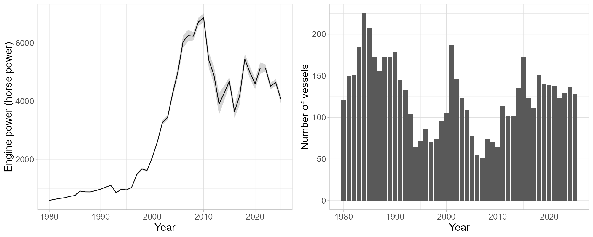
A major restructuring of the Norwegian shrimp fishing fleet towards fewer and larger vessels took place during the late 1990s through the early 2000s (Figure 2). Until 1996, the fishery was conducted using single trawls only until double were introduced. Over the past years, double trawls have been increasingly replaced by triple trawls. An individual vessel may alternate between single and multiple trawling depending on fishing conditions.
Figure 2: Mean engine power (HP) weighted by trawl-time (left) and number of vessels (right) in Norwegian fleet. Data are based on logbook registrations.
The fishery takes place throughout the year but can be seasonally restricted by ice conditions. Fishing activity occurs generally in March to October, with peak activity in May to August.
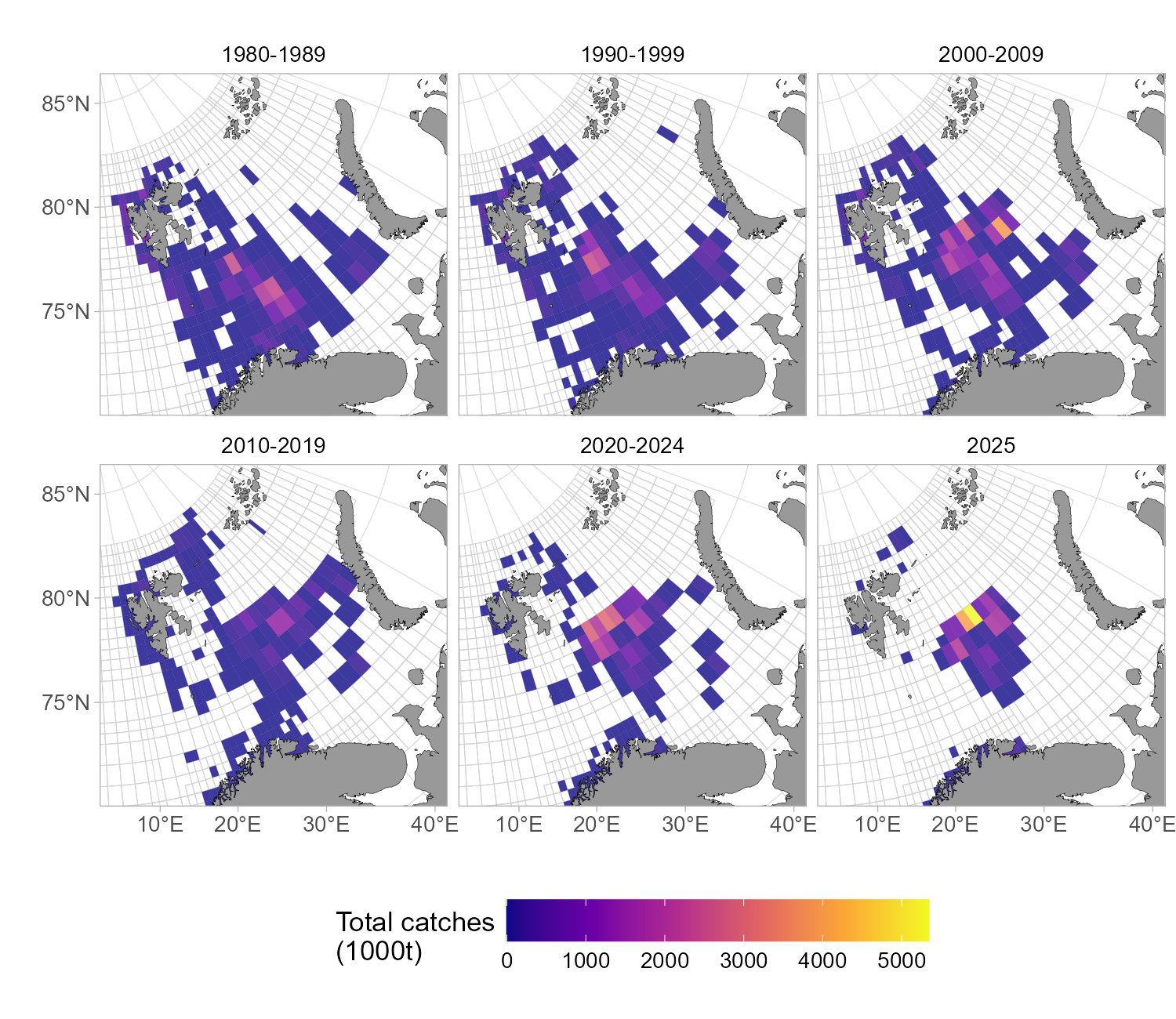
The fishery was previously conducted mainly in the central Barents Sea and on the Svalbard Shelf along with the Goose Bank (southeast Barents Sea). Norwegian logbook data since 2009 show decreased activity in the Hopen Deep and around Svalbard, coupled with increased effort further east in international waters (the “loophole”) (Figure 3). Information from the Norwegian industry points to decreasing catch rates and more frequent area closures due to bycatch of juvenile fish on the traditional shrimp fishing grounds, as well as economic causes as a result of fuel taxation, as the main reasons for the observed change in fishing pattern.
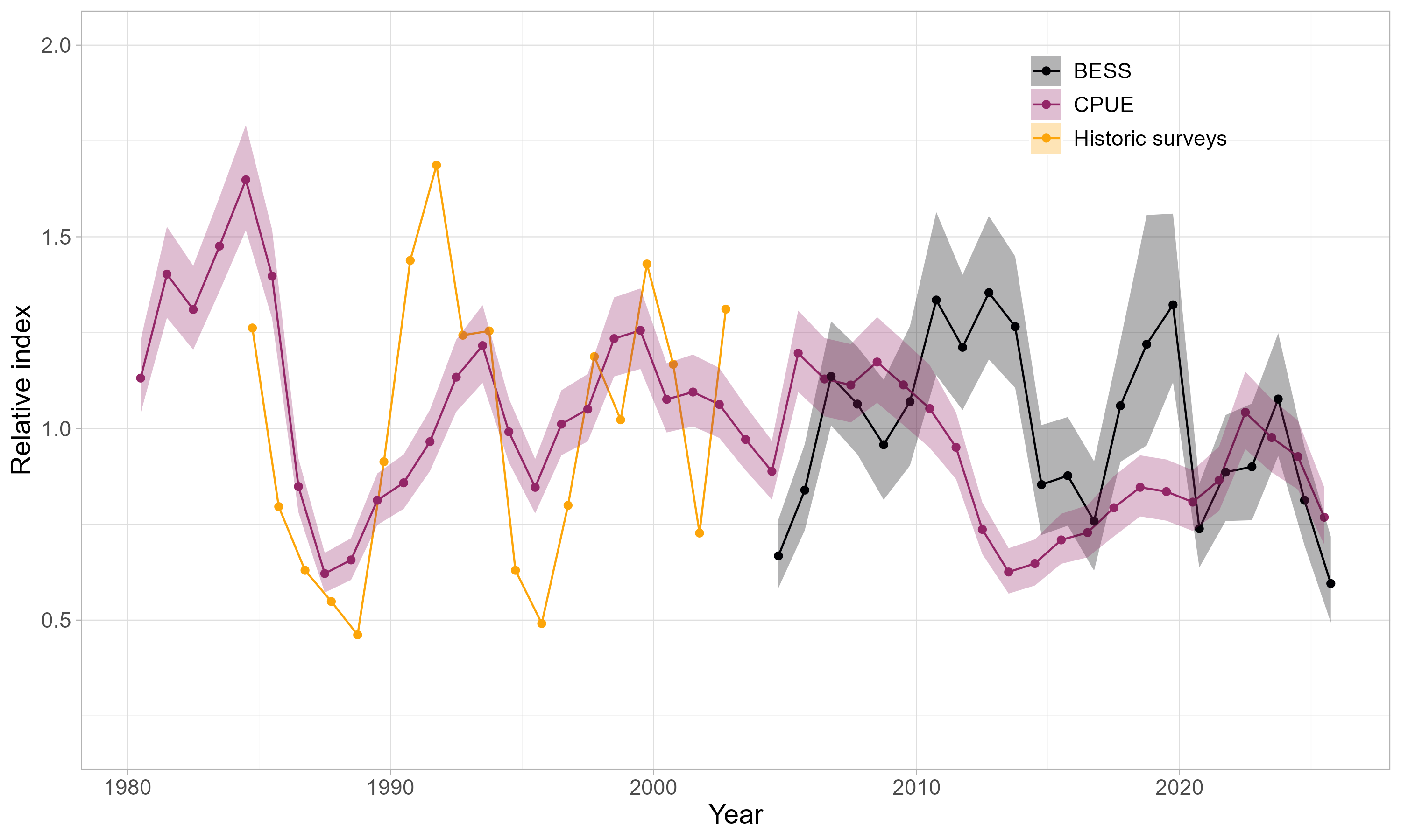
Norwegian logbook data were used in a generalized additive mixed model (GAMM) to calculate a standardized index of catch per unit effort (CPUE) (ICES, 2022c). The GAMM used to derive the CPUE index was implemented in glmmTMB (Brooks et al., 2017) and included the following variables: (1) vessel and (2) area (five survey strata) as random intercepts, (3) season (month) and (4) gear type (single, double or triple trawl) as categorical fixed effects, and vessel size (registered length) as continuous effect with a smooth spline (restricted to 3 knots). The underlying data combines logbook data with lower resolution prior to 2011 with electronic logbooks (ERS) from 2011 onward. The approach estimation method was evaluated and revised during the last benchmark (ICES, 2022c), resolving prior robustness issues and resulting in a stable index (Figure 4). Following the expansion of reporting requirements to vessels below 15 m since 2022, all inshore ERS reportings were removed to avoid potential bias, as the dynamics of inshore stock components are assumed to be not representative for the Barents Sea.
The CPUE index is representative of the exploitable biomass of shrimp ≥15 mm CL, i.e. females and older males. The Norwegian logbook data on which the CPUE index is based represented historically fishing activity from most of the stock’s distribution area. However, the fishery has contracted increasingly into a more limited area in the central Barents Sea in the last decade. Although in recent years the proportion of total catches taken by Norway has varied, it has remained between one third and more than half of the total catches.
The Russian fishery was mainly conducted in the open part of the Barents Sea and the Svalbard area in the past, but later the main fishing grounds shifted eastward near coastal waters of the Novaya Zemlya Archipelago. Catches peaked in 1983–1985 and varied in subsequent years (Figure 1). From 2005 onward, the Russian fishery for shrimp largely ceased and only rebounded 10 years later following a restructuring of the fleet. Russian logbook data since 2023 show increased activity in international waters (Zimmermann et al., 2024). The standardized CPUE index from Russian logbook data showed minor fluctuations from 2017 to 2024 (Zimmermann et al., 2024).
Figure 3: Distribution of annual catches by Norwegian vessels since 1980 based on logbook information. For periods before 2020, mean annual catches across a decade are shown. 2025 includes only data until October.
2.2 - Research survey data
Russian and Norwegian surveys were conducted in their respective EEZs of the Barents Sea from 1984 to 2002 and 1982 to 2004, respectively, to assess the status of the northern shrimp stock. In 2004, these surveys were replaced by the joint Norwegian-Russian Barents Sea Ecosystem Survey (BESS) in August and September, which monitors shrimp along with a multitude of other ecosystem variables in the Barents Sea and around Svalbard (Prozorkevich et al., 2024). In addition, the demersal fish survey in the winter (WS) (Fall et al., 2020) has covered the ice-free parts of the Barents Sea in the beginning of the year since the 1990s, with the inclusion of the Russian EEZ since the 2000s. While designed to survey Atlantic cod and haddock, the winter survey observes northern shrimp on a large proportion of its stations and their catches were recorded consistently over the past two decades.
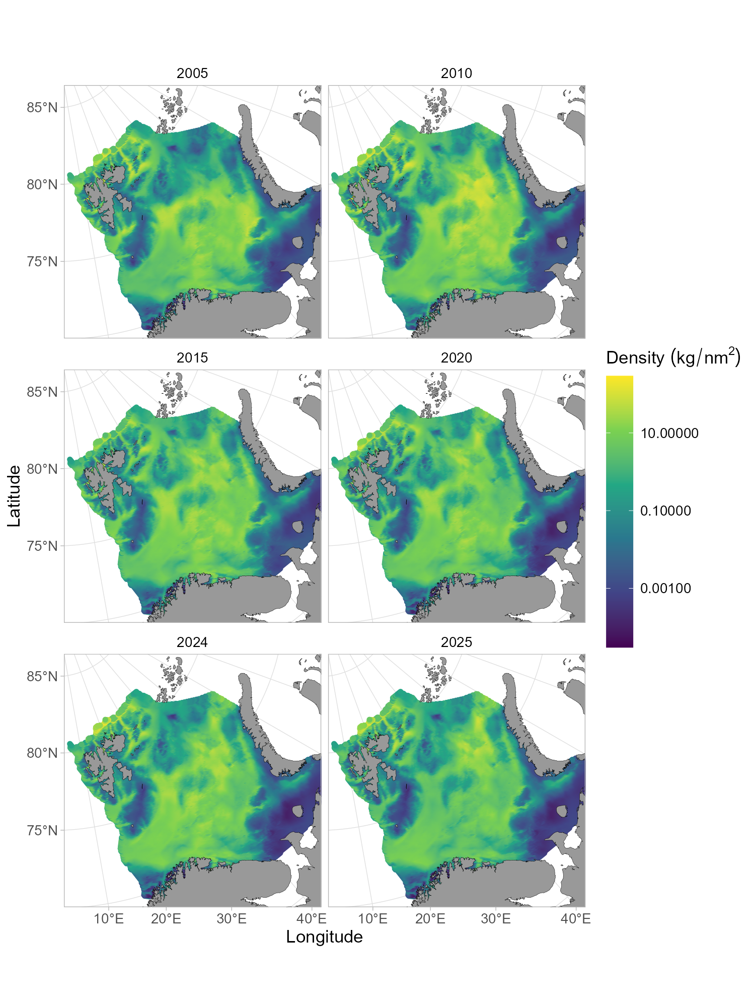
The spatial distribution of shrimp biomass has been relatively stable on a large scale over the recent survey period (Figure 5). In general, the entire survey area of the ecosystem survey (Figure 5) is covered in all years, however, due to heavy ice conditions in 2014 the northern part of the area was not covered, and in 2020 and 2022, parts of the survey were not conducted or at a later stage due to technical problems with survey vessels.
During the benchmark in 2022, estimation methods for the ecosystem survey index were evaluated to determine a more suitable approach for handling incomplete coverage (ICES, 2022c). A model-based approach was subsequently adopted to replace the prior design-based approach, using a GAMM implemented in the R-package sdmTMB (Anderson et al., 2024) that includes spatio-temporal correlation. In the modelled index, missing coverage is predicted out of the estimated relationship between shrimp density and depth as well as the spatio-temporal random fields. The method provides a robust approach that relies on established statistical methodology, provides uncertainty estimates, and improves on the past ad-hoc approaches to produce indices in situations with incomplete coverage. However, it should be noted that the BESS index includes undersized biomass due to inconsistencies in length data due to incomplete length sampling prior to 2022. The index is therefore not strictly representative of exploitable biomass and rather reflects trends in stock biomass, although the difference is assumed to be negligible.
Figure 4: Indices of stock biomass from the (1) joint Russian-Norwegian Barents Sea ecosystem survey (BESS, since 2004), (2) Norwegian logbook data from the fishery (CPUE), and (3) a historic index based on the annual sum of Norwegian shrimp survey and the Russian survey (1984–2002). Lines show the mean estimates, the shaded area the 95% confidence interval. All indices were standardized to their respective mean.
Figure 5: Spatial distribution of shrimp biomass based on ecosystem system survey data. Biomass is predicted with a GAMM including spatio-temporal correlation that was used to produce the standardized survey index.
2.3 - Recruitment indices
The available length data was used to calculate recruitment, defined as abundance of shrimp under 15 mm carapace length. Recruitment was modeled using the same approach as the BESS index, with a GAMM including spatial and spatio-temporal random effects, implemented through the sdmTMB package. Predictions were raised by area and a relative index of recruitment was computed (Figure 6).
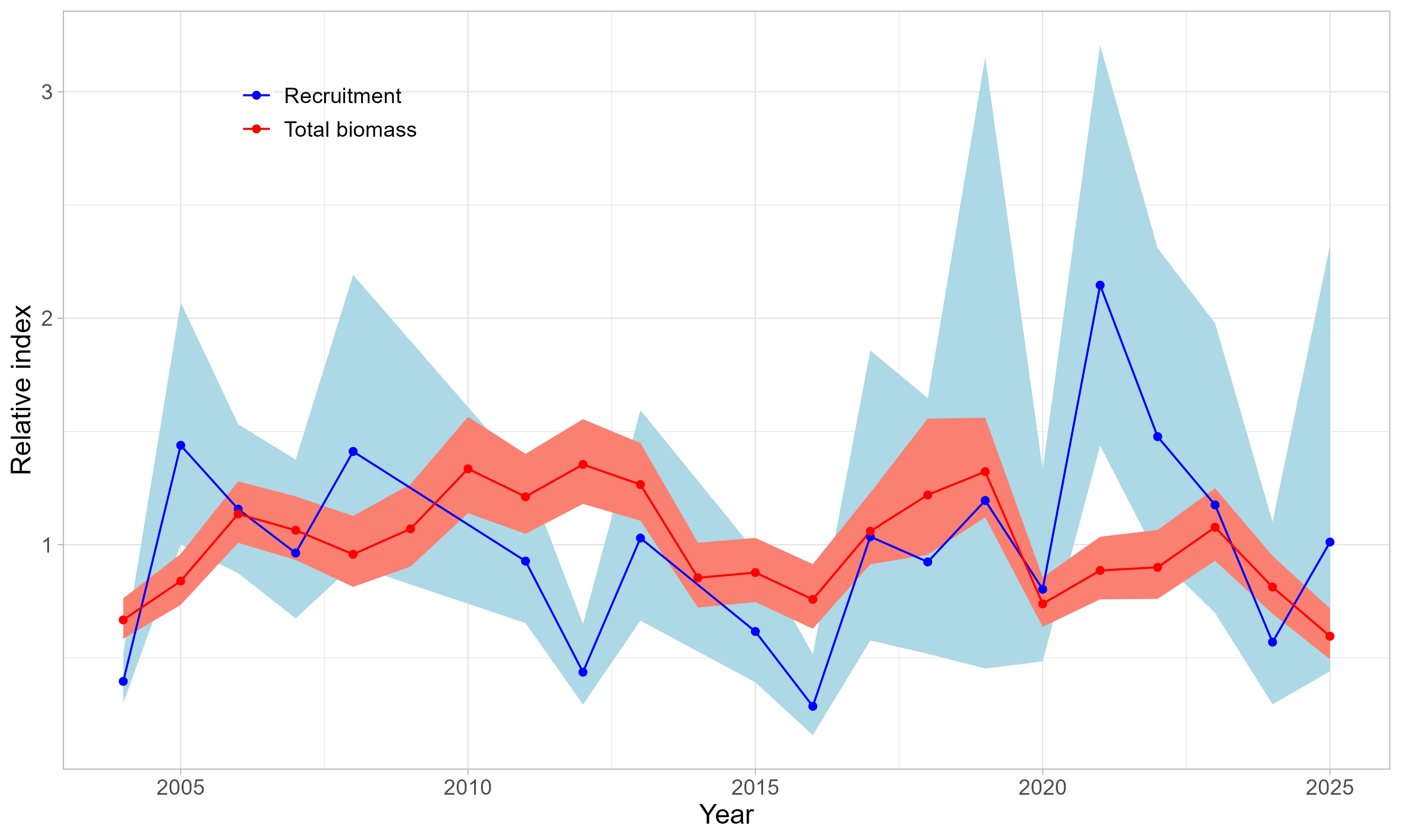
Recruitment showed substantial temporal variation, similar to total biomass. In recent years there has been a particularly pronounced decline, as recruitment decreased from its historical maximum in 2021 to a low level in 2024, before bouncing back to its mean historical value in 2025.
Figure 6: Relative index of recruit abundance (< 15 mm carapace length) and total shrimp biomass from the joint Russian-Norwegian Barents Sea ecosystem survey. Individual data was not available for 2008, 2009 and 2014. Points represent mean estimates per year, lines serve as visual guides for trends, and the shaded area indicates the 95% confidence interval. All indices were standardized to their respective mean.
2.4 - Length indices
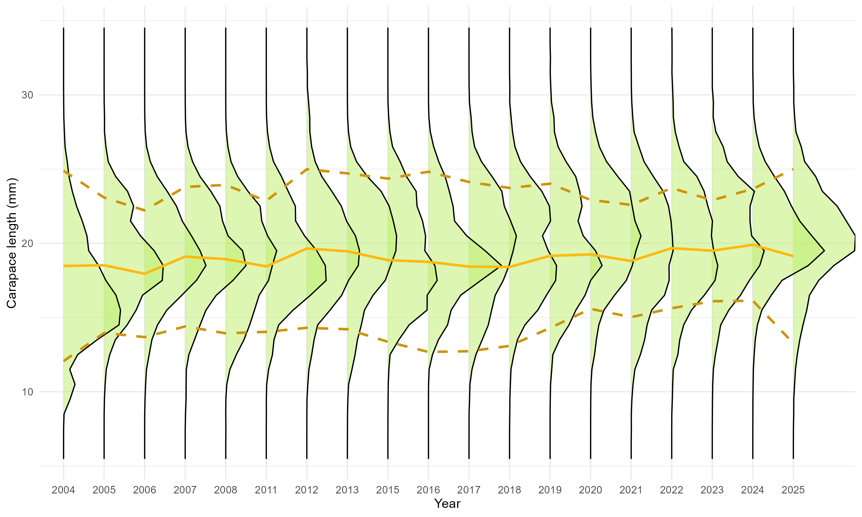
Individual length data has been available through the BESS survey since 2004, except for the years 2009, 2010 and 2014. Across the surveyed period, 32% of stations in average per year were sampled for individual length data, with a mean of 215 shrimps measured per sampled station. Length frequencies were extracted from these individual measurements and subsequently raised to total catch counts to obtain representative length distributions. The temporal evolution of these raised length-frequency distributions is shown in Figure 7.
A spatio-temporal distribution model was then fitted to predict mean shrimp length across the Barents Sea, using depth, hour and year as predictors and spatio-temporal random fields as random effects. Observation error was modeled with a tweedie distribution. Model predictions were aggregated to derive the predicted annual mean shrimp length (solid line in Figure 7).
Overall, mean shrimp length has remained relatively stable throughout the study period, with no clear temporal trend, despite shifts in stock biomass.
Figure 7: Shrimp length frequencies over time with predicted mean (solid line) and standard error (dashed line) overlayed. The years 2009, 2010 and 2014 were omitted because no individual data was available. Shown size range was restricted to <35mm.
2.5 - Reference points
Four reference points are considered: MSY Btrigger and FMSY representing the MSY approach, and Blim and Flim representing the precautionary approach. MSY Btrigger is defined as 50 % of BMSY, and Blim and Flim as 30 % and 170 % of BMSY and FMSY, respectively. BMSY and FMSY are estimated directly in the assessment model.
3 - Assessment
The model is formulated in the state-space framework Surplus production in Continuous Time (SPiCT), implemented in the R package with the same name (Pedersen and Berg, 2017). Within this model, parameters relevant for the assessment and management of the stock are estimated, based on a stochastic version of a surplus-production model.
The configuration implemented in SPiCT in 2022 (ICES, 2022c) was used for the assessment. The model synthesized information from priors, three independent stock indices and the time series of total shrimp catches. The shape of the surplus production function was fixed to a Schaefer-type shape (shape parameter n = 2). Model settings were the same as those determined during the benchmark meeting, with exception of observation error priors and annual weighting added on the inputed stock indices, as well as a prior for growth rate r. Parameter estimates are presented in Table 2.
Description
Parameter
Estimate
Low
High
Log_SE
MSY (kt)
m
99
39
254
4.594
Carrying capacity (kt)
K
1 176
491
2 816
7.070
Catchability CPUE
q1
1.016
0.357
2.889
-6.892
Catchability BESS
q2
1.103
0.386
3.150
-6.810
Catchability historic surveys
q3
0.946
0.330
2.716
-6.963
Observation error CPUE
sdi1
0.119
0.085
0.169
-2.125
Observation error BESS
sdi2
0.150
0.108
0.208
-1.899
Observation error historic surveys
sdi3
0.247
0.192
0.319
-1.398
Table 2: Summary of parameter estimates: mean and 95% confidence intervals for selected parameters estimated in the 2025 assessment. Catchabilities are relative to the stock indices standardized to there mean and were multiplied by 1000 for display purposes.
3.1 - Input time series
The input data consisted of standardized stock indices from time series of fisheries-dependent logbook data for 1980–2025 and trawl-survey biomass indices for 1982–2004, 1984–2005 and for 2004–2025 (Figure 4). The biomass indices of the Norwegian shrimp and Russian surveys were combined into one aggregate index (sum of annual biomass estimates in 1984–2002) assessment input (Figure 4). Catchability parameters for each index, q, were estimated in SPiCT with lognormal observation errors. Total reported catches in ICES Division 1 and 2 since 1970 were used to estimate removals (Figure 1) and, thus, catches were not treated as error-free values. Biomass, B, was estimated relative to the biomass that would yield Maximum Sustainable Yield, BMSY. The estimated fishing mortality, F, refers to the rate of removal of exploitable biomass by fishing and is scaled to the fishing mortality at MSY, FMSY. Model specification, fitting procedure and diagnostics followed the standard recommendations ICES (2024).
3.2 - Priors
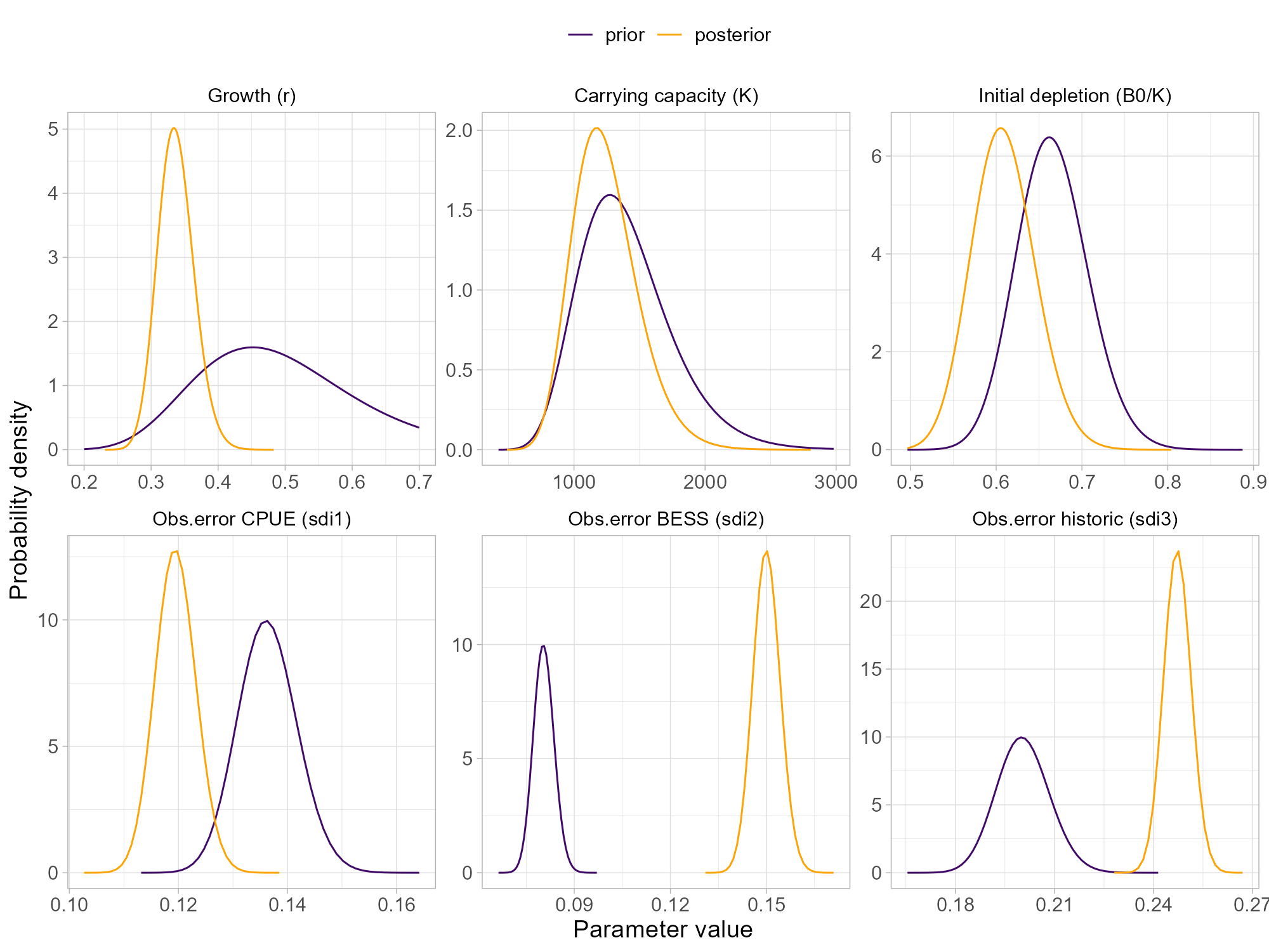
Priors were defined during the benchmark in 2022 for carrying capacity (K) and initial depletion (B0/K) based on a priori knowledge on stock density and historic fishing pressure. To address the issues of low weighting of the survey indices and high dependency on the K prior - as identified in last year’s report (Hvingel and Zimmermann, 2024) - priors on index observation uncertainty and population growth (r), respectively, were introduced. Prior and posterior distributions are shown in Figure 8.
For carrying capacity, a log-normal input prior (7.15 mean ±0.5 SD) was constructed based on the estimates of suitable shrimp habitat in the Barents Sea and carrying capacity in the West Greenland shrimp stock (ICES, 2022c). West Greenland shrimp are comparable to Barents Sea shrimp because of a similar environment, providing a reference value for likely densities at carrying capacity. Together with information habitat size and relative habitat quality, this provided the basis for the K prior. In contrast to past assessments, the K prior was biased-corrected to account for the long upper tail of the log-normal distribution. The r prior was based on information from the meta database www.sealifebase.ca that aggregates information from existing assessment of northern shrimp (-0.79 ±0.5), implemented with a bias-corrected mean. The prior for the initial exploitation level (-0.29 ±0.25, corresponding to a mean of 75 % depletion), on the other hand, was based on information on the historic fishing landings (Melaa et al., 2022) from the Barents Sea prior to the time series included in the assessment.
The standard errors from the GAMMs used to estimate standardized stock indices from the BESS and commercial CPUE data were used to define the priors for the observation errors in SPiCT, informing the assessment model about the uncertainty of the stock indices using extrinsic information from the index estimation and, thus, addressing the issue that the assessment model gave very low weight to the BESS index in the past. For both the CPUE index and the BESS index, the mean estimated standard error of the indices across the respective time series was taken as proxy for CV and therefore set as mean of the observation error prior. For the historic survey time series, no uncertainty estimates were available and, thus, an arbitrary prior (log(0.2) ± 0.2) was used for the observation error. Furthermore, because the mean standard error of the CPUE index was considered too low compared to the BESS index, it scaled up to a similar magnitude as the BESS index. This represents an ad-hoc solution that requires further investigation into the low uncertainty of the CPUE index. In addition, the prior for catch observation error was set to log(0.1) as default, and subsequently the link between observation and process errors (alpha and beta parameters) was deactivated as recommended by ICES (ICES, 2024).
Figure 8: Prior and posterior distribution for carrying capacity K, growth rate r, initial depletion B0/K, and observation errors of commercial CPUE, BESS historic surveys indices.
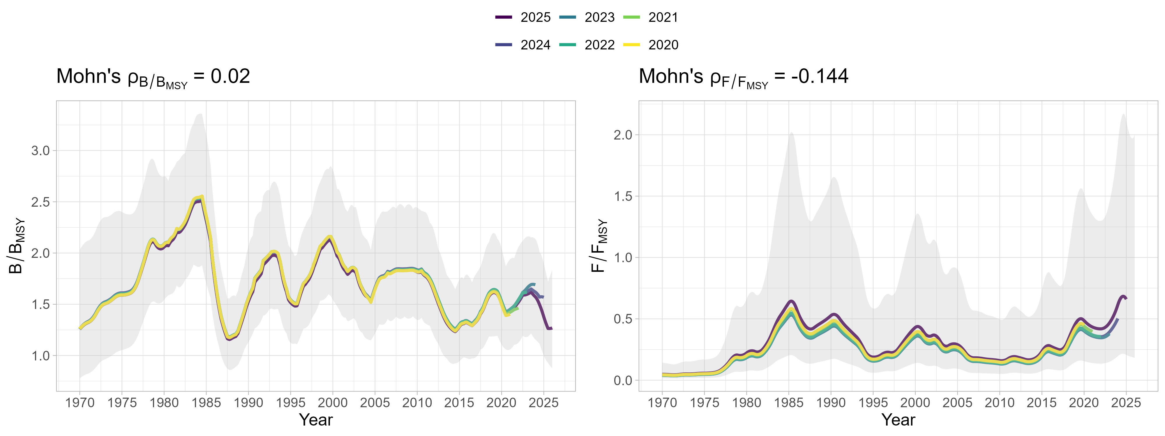
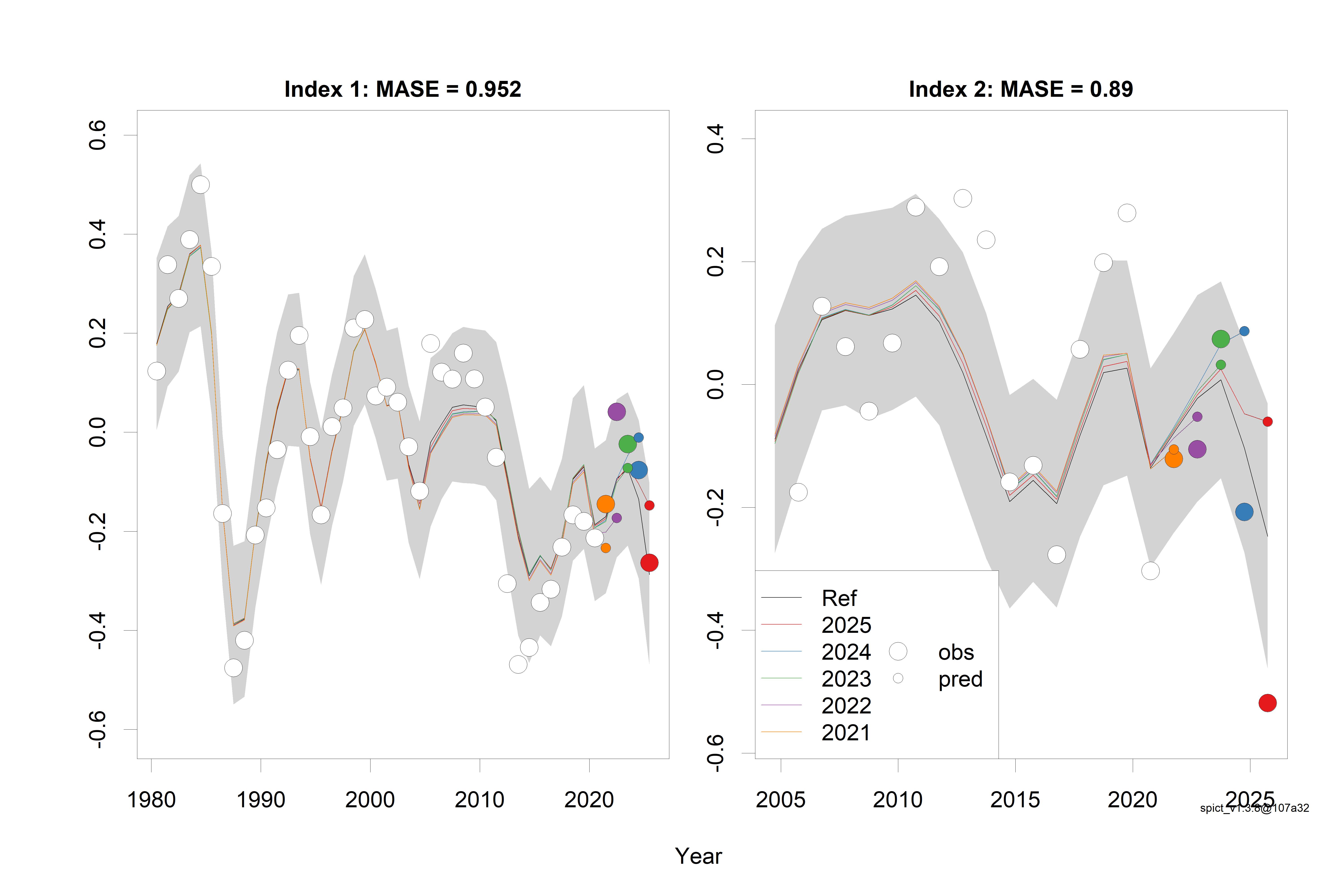
3.3 - Model performance
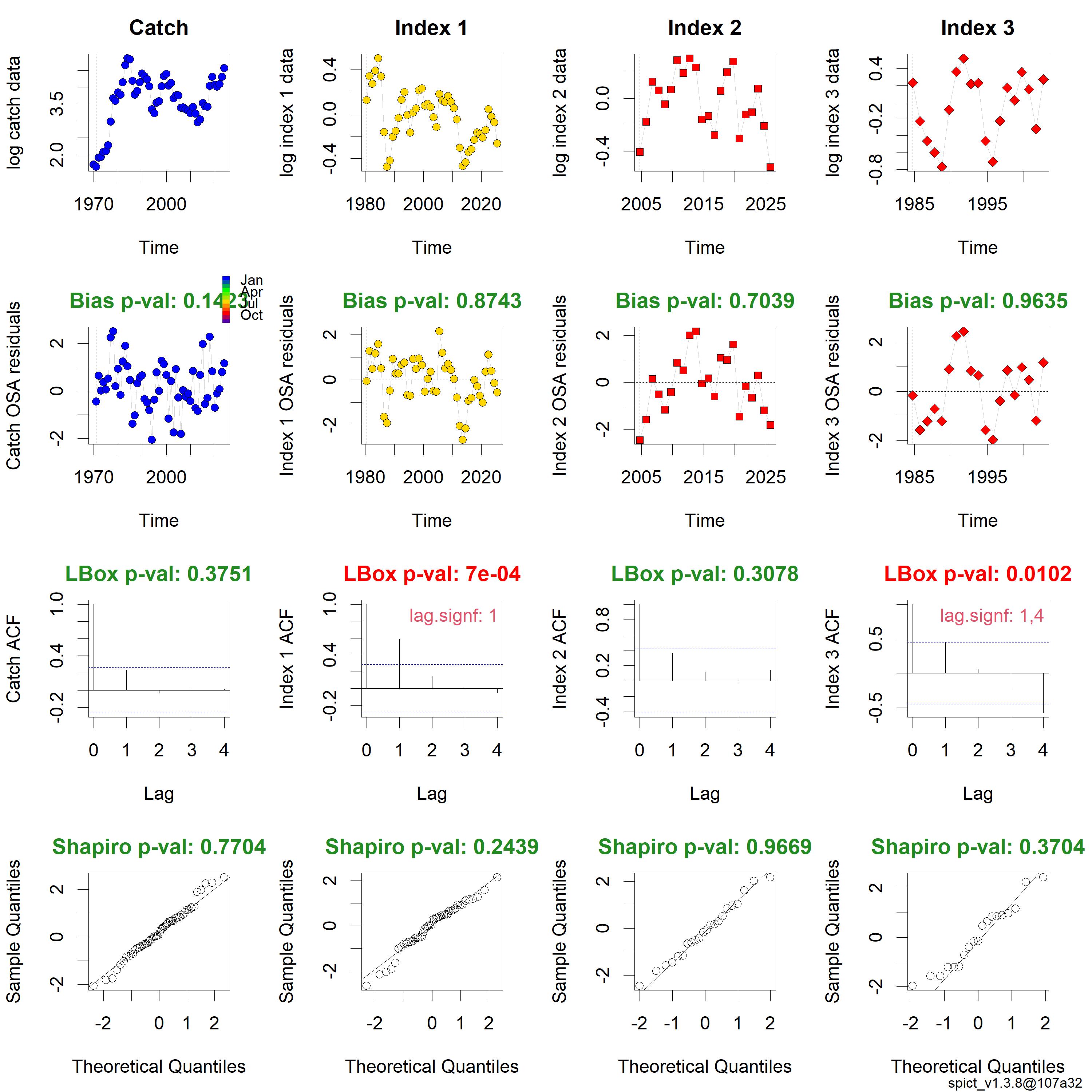
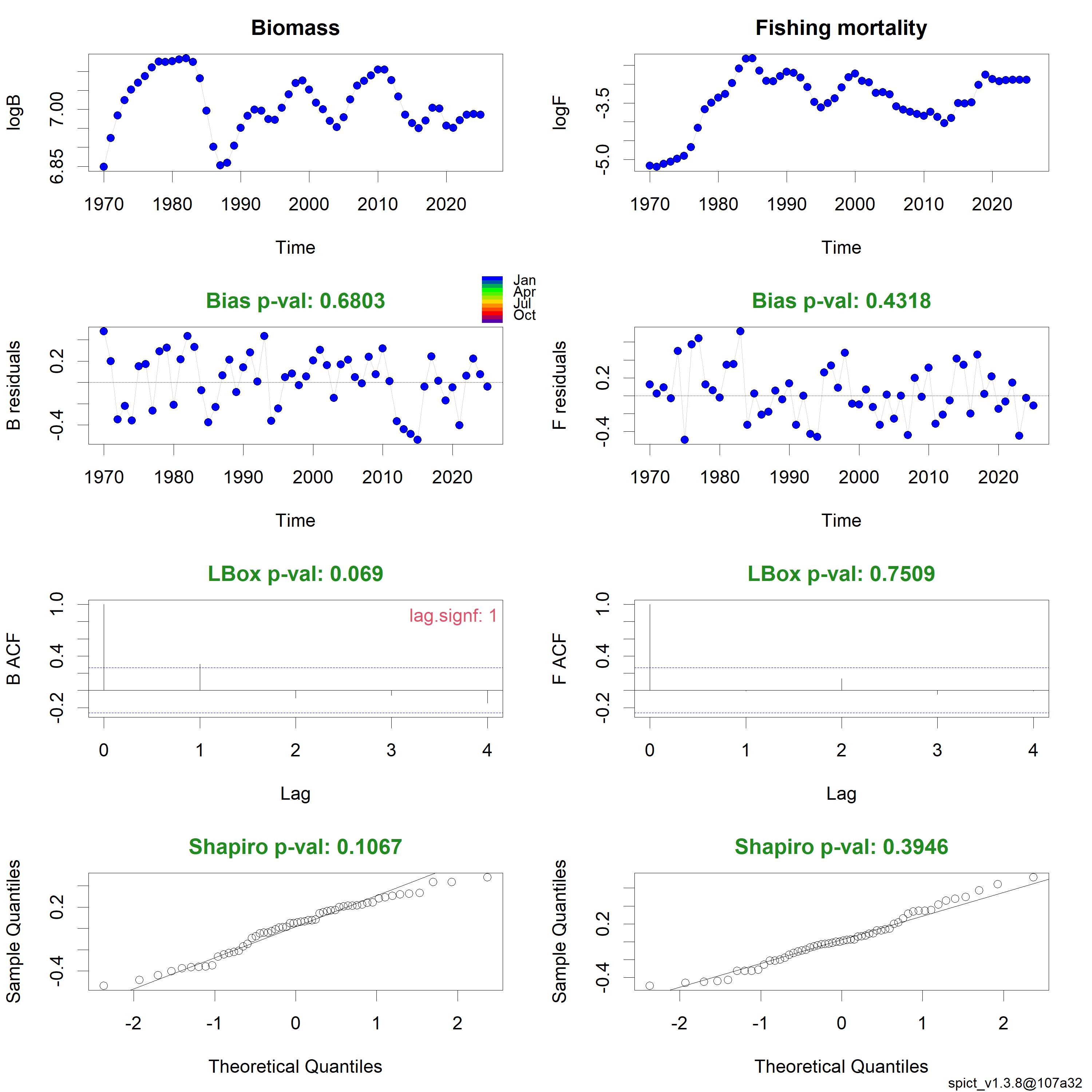
The model was validated and performed generally well, in line with the in-depth exploration and sensitivity analysis conducted during the benchmark (ICES, 2022c). The model converged, was stable (<1 % deviating estimates in jitter analysis), showed very little retrospective bias (Figure 9), had low mean absolute scale error (MASE < 1) (Figure 10), and fulfilled most acceptance criteria in terms of residual patterns of observation and process errors (see annex) and uncertainty. Minor violations were caused by relatively large uncertainty in the F/FMSY estimates, reflecting the lack of contrast in the time series, and correlated one-step-ahead residuals of the stock indices.
The observation error priors and annual multiplier introduced in this year’s assessment resolved the previous issue of problematic residual patterns and little to no weight given to the survey indices, instead balancing the weighting between BESS and CPUE index. However, this only shifted the minor issue with the residual patterns of input indices from the survey indices (Hvingel and Zimmermann, 2024) to the CPUE index. Although the changes implemented in this year’s assessment reduce the extent of previous issue by reducing the dominance of the CPUE index, the model is not capable of fully resolving the diverging trends of survey and CPUE indices in parts of the time series. Potential reasons are that the CPUE index currently does not account sufficiently well for technological creep and spatial contractions in the fishery, underlining the need for further investigations into the CPUE standardization.
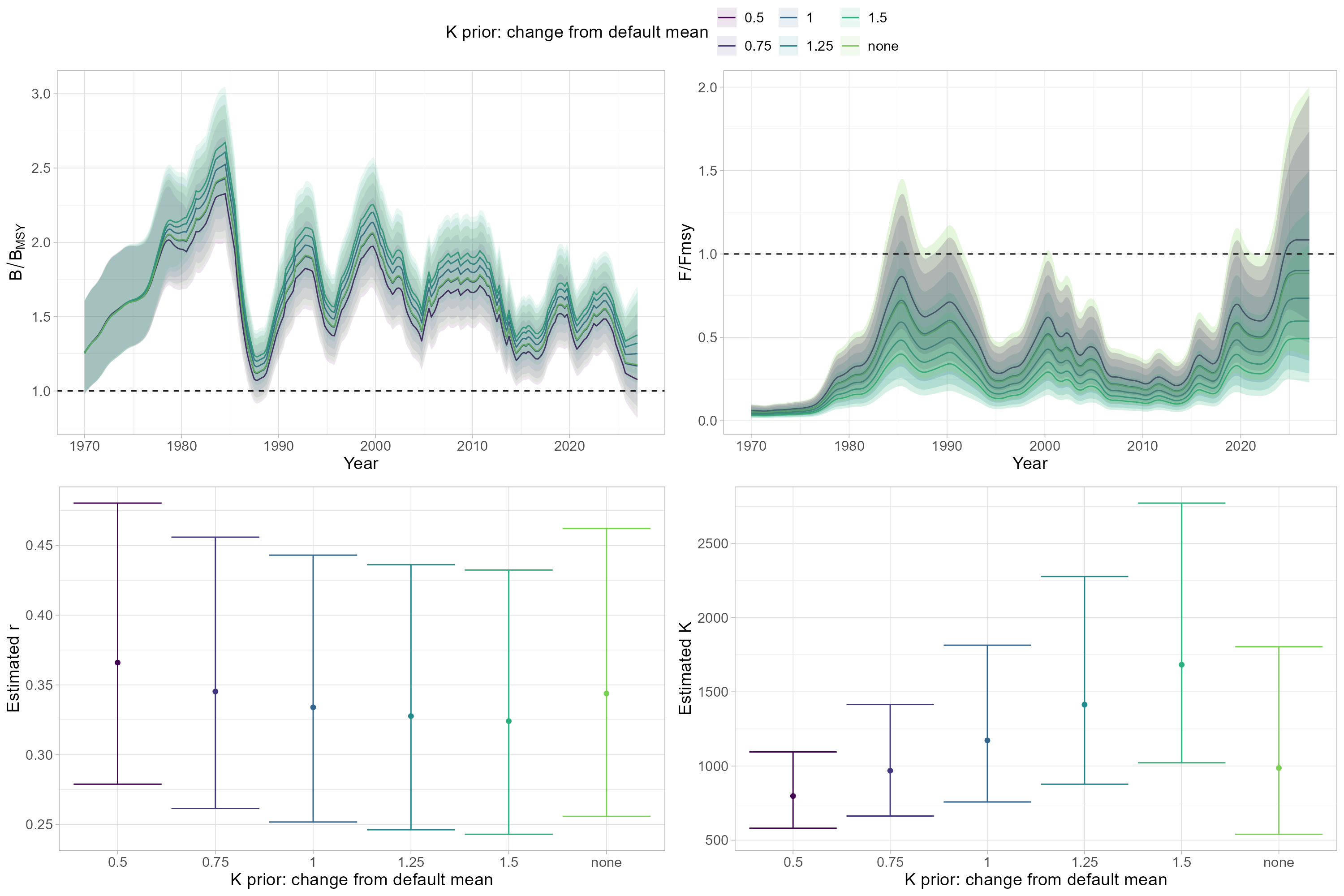
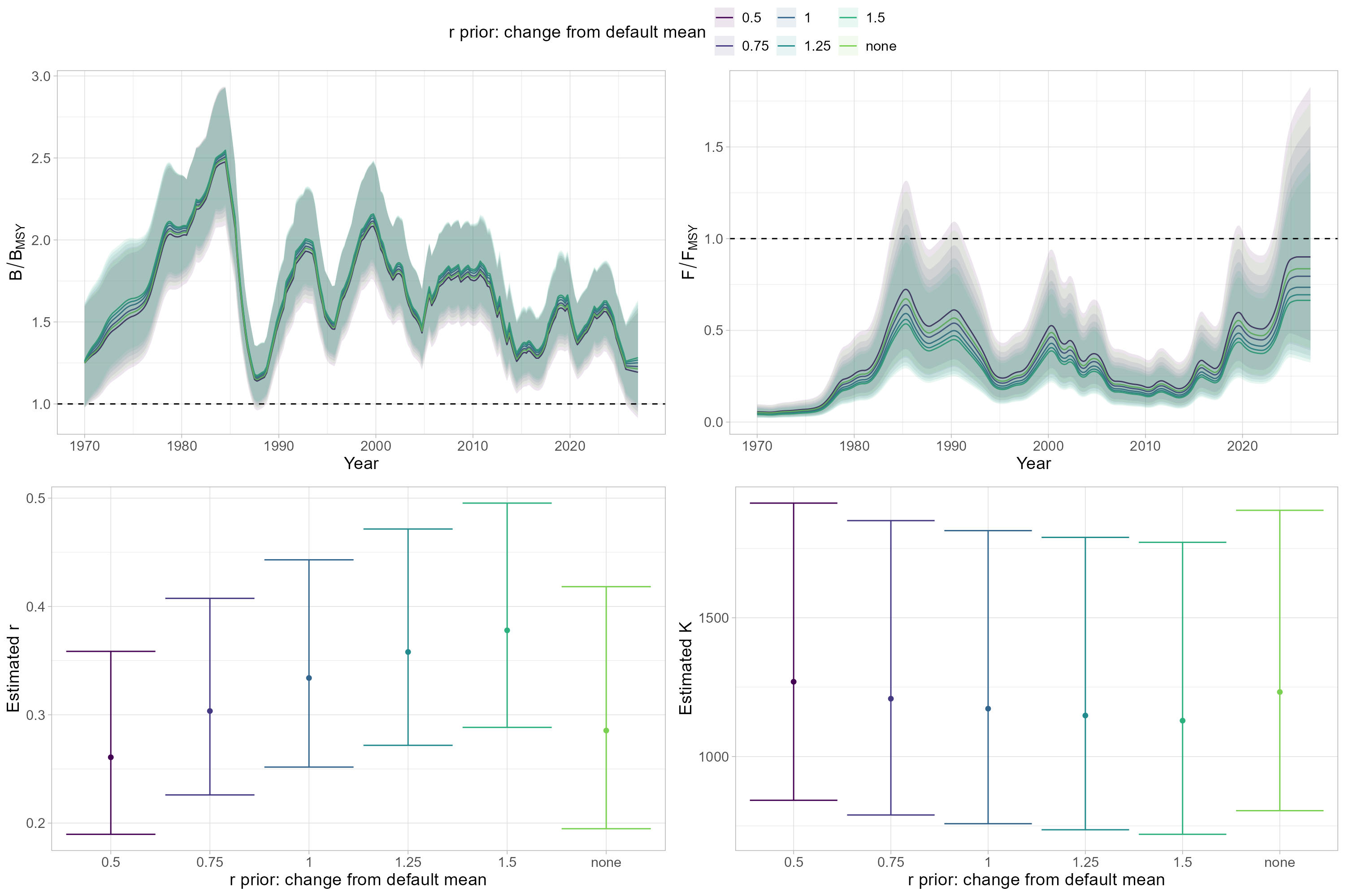
The sensitivity of the stock and parameter estimates was explored during the benchmark in 2022 (ICES, 2022c). The analysis showed that the prior definition for initial depletion had no impact on the perception of stock status. This conclusion still applies and includes also the new prior on r. However, as noted in the benchmark report, there is some sensitivity of the stock trends to the mean of the K prior. While not resulting in a clear impact on the state of the stock, this indicates nevertheless that the definition of the K prior is a key element of the assessment and should be therefore carefully re-evaluated in the future.
Figure 9: Retrospective analysis of the assessment model with 5 peels back in time from the current assessment year. Shown are resulting estimates in F/FMSY and B/BMSY with their respective Mohn’s rho values.
Figure 10: Hindcast of the assessment models for the stock indices from commercial CPUE (index 1) and BESS (index 2) with 5 years back in time from the current assessment year. Shown are observed index estimates vs. model predictions, and the corresponding MASE.
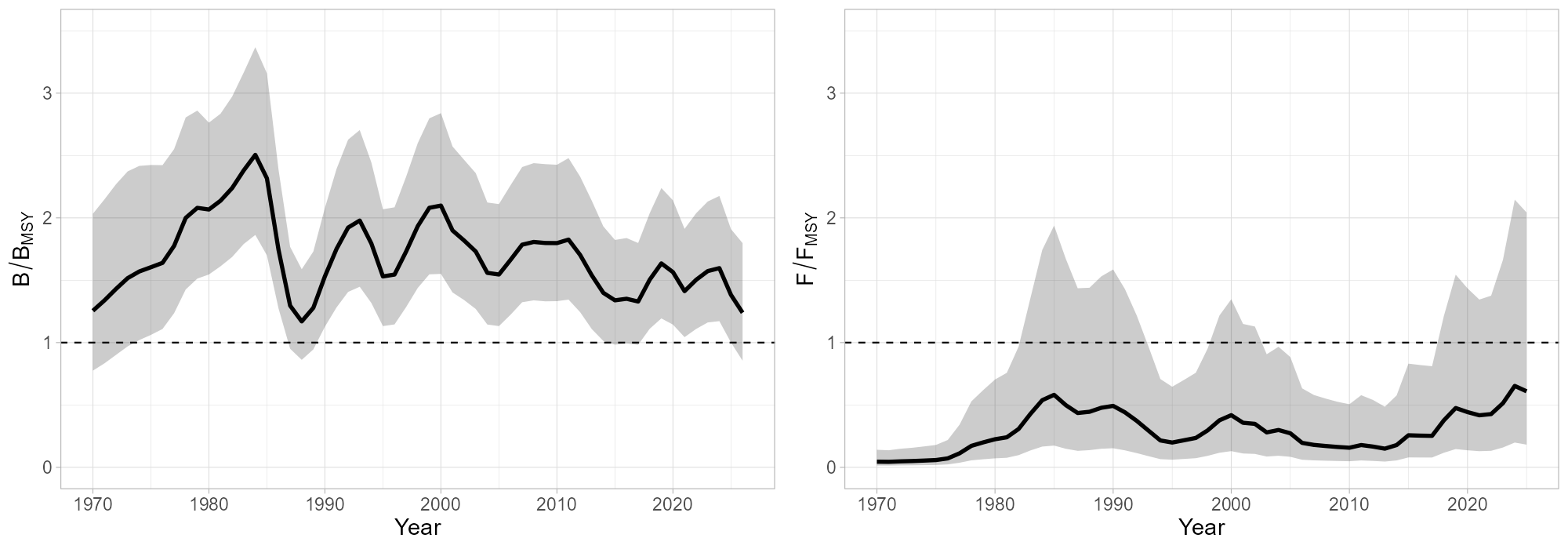
3.4 - Stock size and fishing mortality
Exploitable stock biomass was estimated to above BMSY for the entire time series since 1970 (Figure 11). The lowest biomass level in the mid-1980s occurred following some years with high catches. Since then, the stock has varied around a stably level above BMSY. The corresponding mean estimate of fishing mortality has remained below FMSY throughout the history of the fishery, with only three periods during the 1980s, around 2000 and since 2018 that the estimates indicate a (low) probability of exceeding FMSY. For assessment year 2025, there is a significant probability that fishing mortality was above FMSY, whereas there is still less than 1 % probability that exploitable biomass was below MSY Btrigger in the beginning of 2026 (Table 3).
Figure 11: Estimated relative biomass (B/BMSY) and fishing mortality (F/FMSY) for 1970-2025. Solid lines represent the mean estimates, shaded surfaces the 95% confidence intervals. BMSY and FMSY are indicated with dashed lines.
2025
2026
Exploitable stock biomass (B/BMSY )
1.39
1.24
Fishing mortality (F/FMSY )
0.64
0.71
Probability of falling below MSY Btrigger
<0.1
<0.1
Probability of falling below Blim
<0.1
<0.1
Probability of exceeding FMSY
23
30
Probability of exceeding Flim
5.4
8.3
Table 3: Estimates of relative exploitable stock biomass and fishing mortality as well as exceeding reference points in 2025 and 2026 at the beginning of each year.
3.5 - Forecast and management plan
An intermediate year catch constraint based on the predicted catches for 2025 was used to forecast the catch scenarios in SPiCT. The forecasts for all catch scenarios were produced with the manage function in SPiCT for the advice period 2026–2027, including the predicted catch in 2025 as catch constraint for the intermediate year. For the advice, a short-term forecast is produced from the fitted stock assessment model using the fractile rule (35th percentile).
A management strategy evaluation for shrimp in the Barents Sea was conducted in 2024 (Trochta et al., 2024) and four of the evaluated harvest control rules (HCR) were proposed as suitable basis for a management plan (IMR-PINRO, 2024). All four accepted HCRs used FMSY or a fraction (90 or 80 %) thereof as target F and a linear decrease of F below MSY Btrigger (0.5 BMSY) to zero at Blim (0.3 BMSY). The management plan was discussed at the autumn meeting of the Norwegian-Russian fisheries commission in 2024, but no HCR was adopted. The current advice for shrimp in the Barents Sea was therefore produced on a generic basis, using a precautionary MSY approach. However, the previously used FMSY mode was replaced with the 35th percentiles of the catch, F/FMSY and B/BMSY distributions under FMSY, following recommendation of ICES on catch advice for stocks using a SPiCT assessment (Berg et al., 2021). For comparison, additional catch scenarios presented are fishing mortality at FMSY (mean of catch distribution), the same level as in assessment year 2025, and zero fishing. The catch resulting precautionary MSY approach is line with recent maximum catches, whereas fishing at FMSY are minor (Table 4) would imply a substantial increase in fishing pressure.
Scenario
Catch (2026)
B2027/BMSY
F2026/FMSY
% risk of B2027 < MSY Btrigger
% risk of F2026 > FMSY
% risk of F2026 > Flim
MSY approach *
83
1.25
0.71
<0.1
30
9.2
F2026 = FMSY
113
1.20
1.00
<0.1
50
21
F2026 = F2025
68
1.28
0.58
<0.1
20
5
F2026 = 0
0
1.39
0.00
<0.1
<0.1
<0.1
* Using the fractile rule with 35th percentiles of F/FMSY and B/BMSY distributions and the catch distribution under F=FMSY
Table 4: Northern shrimp in ICES subareas 1 and 2. Annual catch scenarios for 2026. Catches are in thousand tonnes, exploitable biomass and fishing mortality are relative values, and risks are in percentages.
4 - Environmental and other considerations
4.1 - Temperature
In the ecosystem survey, shrimps were only caught in areas where bottom temperatures were above 0°C. Highest shrimp densities were observed between zero and 4°C, while the limit of their upper temperature preference appears to lie at about 6-8°C. Although temperature is a likely driver for stock dynamics and distribution, no relationship of temperature with observed catch rates or stock biomass could be found during analysis conducted at the benchmark (ICES, 2022c). Further investigations of environmental drivers of shrimp distribution and abundance are necessary.
4.2 - Predation
Both stock development and the rate at which changes might take place can be affected by changes in predation, in particular by Atlantic cod, which has been documented as capable of consuming large amounts of shrimp. The relationship between shrimp biomass and cod biomass has been investigated during the benchmark but was not found to be significant given the available data (ICES, 2022c). The cod stock in the Barents Sea increased to historically very high levels during the past decade but has since decreased substantially in a significant trend reversal, providing a strong contrast for further analysis. As predator biomass may not be representative of predation pressure, further investigations into shrimp consumption by cod and potential impacts on stock dynamics are recommended.
4.3 - Recruitment, and reaction time of the assessment model.
The model used is best at projecting trends in stock development but estimates and uses long-term averages of stock dynamic parameters. Large and/or sudden changes in recruitment or mortality may therefore be underestimated in model predictions.
5 - Research recommendations
The fishery has expanded since 2014 and catches by countries other than Norway have increased to account for more than 50% of the total in most years. In 2016, NIPAG therefore recommended that available data (logbook data and catch samples) from the participating nations be made available for the assessment. An ICES data call has been made and some parties have now provided aggregated data on total catch and effort. Because of the low resolution of the data and short time series, it is currently not suitable for producing a standardized LPUE index and has therefore been of limited use in the assessment work. Further data requests and analysis of available data sources, including RDBES, are recommended. Receiving good information on catches of the EU in the assessment year would be of particular importance, considering their increased importance in the fishery.
During the 2024 assessment, the weighting issue that resulted in negligible influence of the BESS index on stock estimates has been resolved, resulting in a more balanced weighting of stock indices. Considering that the survey coverage of the stock is comprehensive and representative, this is considered a major improvement. However, the lack of alignment between the trends of survey and commercial CPUE indices remains a potential issue for the assessment and a source of uncertainty. It is therefore recommended to continue the re-evaluation of stock indices from the 2022 benchmark, focusing on 1) the standardization of commercial CPUE over time, especially in light of a spatial contraction of the fishery that is not fully accounted for in the current index; 2) the potential use of data from the demersal fish survey in winter for a stock index to provide relevant information on the stock development within the assessment year (ICES, 2022c), especially given that BESS data is often still incomplete at the time of the assessment; and 3) re-estimating the historic survey index from the original Norwegian and Russian shrimp survey data to standardize methodology, increase comparability with the BESS index and produce uncertainty estimates.
Despite the long time series of the assessment, the lack of contrast causes a dependency on informative priors. The carrying capacity prior in particular has a relevant effect on stock estimates. The prior definition and the sensitivity of the assessment to them should be therefore routinely evaluated. Furthermore, it is recommended to test a loosening of priors, notably carrying capacity.
The seasonality of the fishery is currently not included in the assessment model, although SPiCT is a continuous time framework that allows for modelling seasonality of catches explicitly. The current configuration sets the timing of the stock indices to the month of the year where they, in average, originate from, but treats catches as annual, discrete quantity. However, most fishing activity takes place in summer, creating strong fluctuations in fishing pressure throughout the year that should be accounted for. Further analysis of the demersal fish survey in winter could provide insights on the in-year dynamics of the stock, as it provides a fishery-independent data early in the year before the fishery takes place, whereas the BESS survey in autumn reflects the state of the stock after a large proportion of the annual catches have been taken. Preliminary research along these lines indicates that incorporating additional winter survey data could improve the current assessment by enhancing the predictive accuracy of the SPiCT model (Casla, 2025).
During the 2022 benchmark, it was recommended to investigate further the predator-prey relationship between shrimp and cod, including available data from cod stomach sampling. This recommendation has gained relevance since then due to the significant decrease of the cod stock, possibly reducing the predation pressure and counteracting an increase in fishing activity. Estimating overlap between shrimp and cod distribution as well as shrimp consumption of cod and incorporating this information into the assessment could result in a relevant improvement of the assessment quality and provide a stepping stone towards a more ecosystem-based management of the stock.
Only the exploitable biomass of the stock is currently assessed, cohort and recruitment dynamics remain unaccounted for in the stock assessment model. Options to incorporate information on population dynamics into the assessment should be investigated, for instance in form of size-based indicators. Catch sampling could in this context provide relevant data and should be re-considered.
The current stock definition includes all shrimp north of 62⁰N. Besides shrimp in the Barents Sea, this also covers inshore populations along the Norwegian coast and inside of fjords, as well as the shelf edges north and west of Svalbard. Especially the latter should likely be treated as separate stock components that with their own dynamics, possibly at the level of each fjord. Furthermore, there are clear distinctions in the fleet structure and dynamics between the large freezer vessels fishing offshore in the Barents Sea, and the smaller coastal vessels producing mostly fresh cooked shrimp for the local market. Although catches from the coastal component are marginal compared to the Barents Sea, combining information from the different areas and stock components might increase the risk for biased signals. This was underlined by the impact of increased logbook reporting from the smaller coastal vessels on the CPUE index. Further research of the stock structure and exploring separate assessments or area-based approaches to differentiate the stock and fleet components better is therefore recommended.
A recent study highlighted that maximum economic yield for the stock is likely significantly lower than MSY (Lancker et al., 2023), emphasising that economic factors are likely limiting the fishery. The economic drivers of fisheries dynamics could provide insights on economically optimal harvest strategies. The management strategy evaluation conducted in 2024 (Trochta et al., 2024) provided a comprehensive simulation framework to test management strategies but did not include economic components. It is therefore recommended to expand the simulation framework with an economics component to improve our understanding of the fishery dynamics and develop economic performance indicators and reference points.
6 - References
Anderson, S. C., Ward, E. J., English, P. A., Barnett, L. A. K., and Thorson, J. T. 2024. sdmTMB: An r package for fast, flexible, and user-friendly generalized linear mixed effects models with spatial and spatiotemporal random fields. bioRxiv: 2022.03.24.485545. https://www.biorxiv.org/content/biorxiv/early/2024/07/18/2022.03.24.485545.full.pdf.X
Berg, C., Coleman, P., Cooper, A., Hansen, H. Ø., Haslob, H., Herrariz, I. G., Kokkalis, A., et al. 2021. Benchmark workshop on the development of MSY advice for category 3 stocks using surplus production model in continuous time; SPiCT (WKMSYSPiCT).
Brooks, M., Kristensen, K., Benthem, K. van, Magnusson, A., Berg, C. W., Nielsen, A., Skaug, H. J., et al. 2017. glmmTMB balances speed and flexibility among packages for zero-inflated generalized linear mixed modeling. The R Journal, 9: 378–400. https://journal.r-project.org/archive/2017/RJ-2017-066/index.html.X
Casla, A. R. 2025. Effects of environmental conditions and seasonality on barents sea shrimp dynamics and consequences for stock assessment. University of the Algarve, Faro, Portugal. http://hdl.handle.net/10400.1/27663.X
Fall, J., Wenneck, T., Bogstad, B., Fuglebakk, E., Gjøsæter, H., Seim, S. E., Skage, M. L., et al. 2020. Fish investigations in the barents sea winter 2020. IMR/PINRO Joint Rep Ser, 2020: 1–99.
Lancker, K., Voss, R., Zimmermann, F., and Quaas, M. F. 2023. Using the best of two worlds: A bio-economic stock assessment (BESA) method using catch and price data. Fish and Fisheries. https://onlinelibrary.wiley.com/doi/abs/10.1111/faf.12759.X
Melaa, K. W., Zimmermann, F., Søvik, G., and Thangstad, T. H. 2022. Historic landings of northern shrimp (Pandalus borealis) in norway - data per county for 1908-2021. Rapport fra havforskningen, 2022. https://www.hi.no/hi/nettrapporter/rapport-fra-havforskningen-en-2022-24 .X
Prozorkevich, D., Eriksen, E., Karlson, S., Trofimov, A., Ingvaldsen, R. B., Grøsvik, B. E., Prokhorova, T., et al. 2024. Survey report (part 2) from the joint norwegian/russian ecosystem survey in the barents sea and the adjacent waters august-october 2023—marine environment, mesozooplankton, commercial demersal fish, fish biodiversity, commercial shellfish, benthic invertebrate community, marine mammals and seabirds. IMR/PINRO Joint Report Series.
Table 5: Catches in tonnes, as used for the assessment by fleet. Catches for the final year are based on preliminary information, and country-specific information only available from 2000 (except for Norway and Russia).
Year
BESS index
Historic index
CPUE index
Catch
1970
6
1971
5
1972
7
1973
7
1974
8
1975
8
1976
10
1977
20
1978
39
1979
36
1980
1.13
46
1981
1.40
44
1982
1.31
63
1983
1.48
105
1984
1.26
1.65
128
1985
0.80
1.40
124
1986
0.63
0.85
65
1987
0.55
0.62
43
1988
0.46
0.66
49
1989
0.91
0.81
63
1990
1.44
0.86
81
1991
1.69
0.97
75
1992
1.24
1.13
69
1993
1.25
1.22
56
1994
0.63
0.99
28
1995
0.49
0.85
25
1996
0.80
1.01
35
1997
1.19
1.05
36
1998
1.02
1.23
56
1999
1.43
1.26
76
2000
1.17
1.08
81
2001
0.73
1.10
57
2002
1.31
1.06
61
2003
0.97
39
2004
0.67
0.89
43
2005
0.84
1.20
43
2006
1.14
1.13
30
2007
1.06
1.11
30
2008
0.96
1.17
28
2009
1.07
1.11
27
2010
1.34
1.05
25
2011
1.21
0.95
30
2012
1.35
0.74
25
2013
1.27
0.63
19
2014
0.85
0.65
21
2015
0.88
0.71
34
2016
0.76
0.73
31
2017
1.06
0.79
30
2018
1.22
0.85
56
2019
1.32
0.84
74
2020
0.74
0.81
58
2021
0.89
0.86
55
2022
0.90
1.04
60
2023
1.08
0.98
74
2024
0.81
0.93
95
2025
0.60
0.77
71
Table 6: Northern shrimp in subareas 1 and 2. Input data for the stock assessment model.
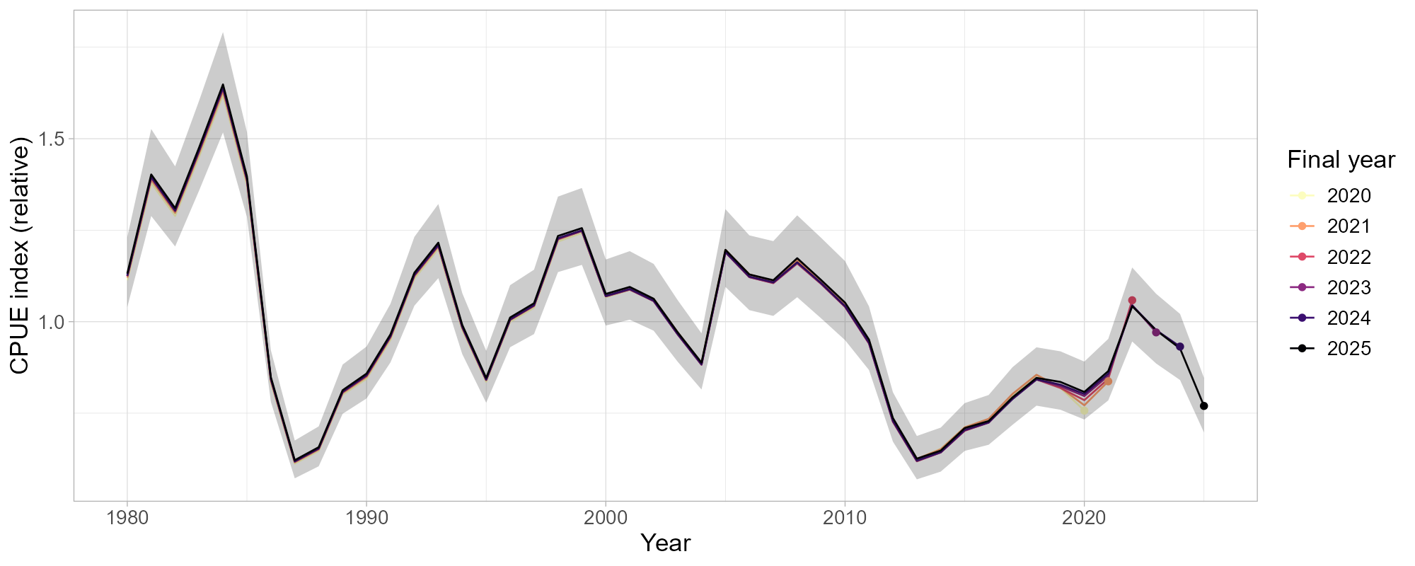
Figure 12: Retrospective analysis of the standardized CPUE index based on Norwegian data. The solid black line shows the index used in the current assessment, and colored lines retrospective indices with data restricted to January-October in the final year, peeling off years back to 2015. Index values are centered around the mean of the series. The shaded area marks the 95% confidence intervals. Indices were standardized using a GAMM implemented in glmmTMB.
7.2 - Model diagnostics
Figure 13: One-step-ahead residuals of the stock assessment model for the time series of catch, commercial CPUE (index 1), BESS (index 2) and historic surveys (index 3).
Figure 14: Residuals of the stock assessment model for the process errors of biomass and fishing mortality.
Figure 15: Sensitivity of model estimates of B/BMSY, F/FMSY, r and K to the mean of the K prior distribution. Included are model runs where K prior mean was varied between 50 and 150% of the final model configuration, as well as a model run without K prior (“none”). Shown are esti-mated means (lines/dots) and 95% confidence intervals (shaded areas/error bars).
Figure 16: Sensitivity of model estimates of B/BMSY, F/FMSY, r and K to the mean of the r prior distribution. Included are model runs where r prior mean was varied between 50 and 150% of the final model configuration, as well as a model run without r prior (“none”). Shown are esti-mated means (lines/dots) and 95% confidence intervals (shaded areas/error bars).
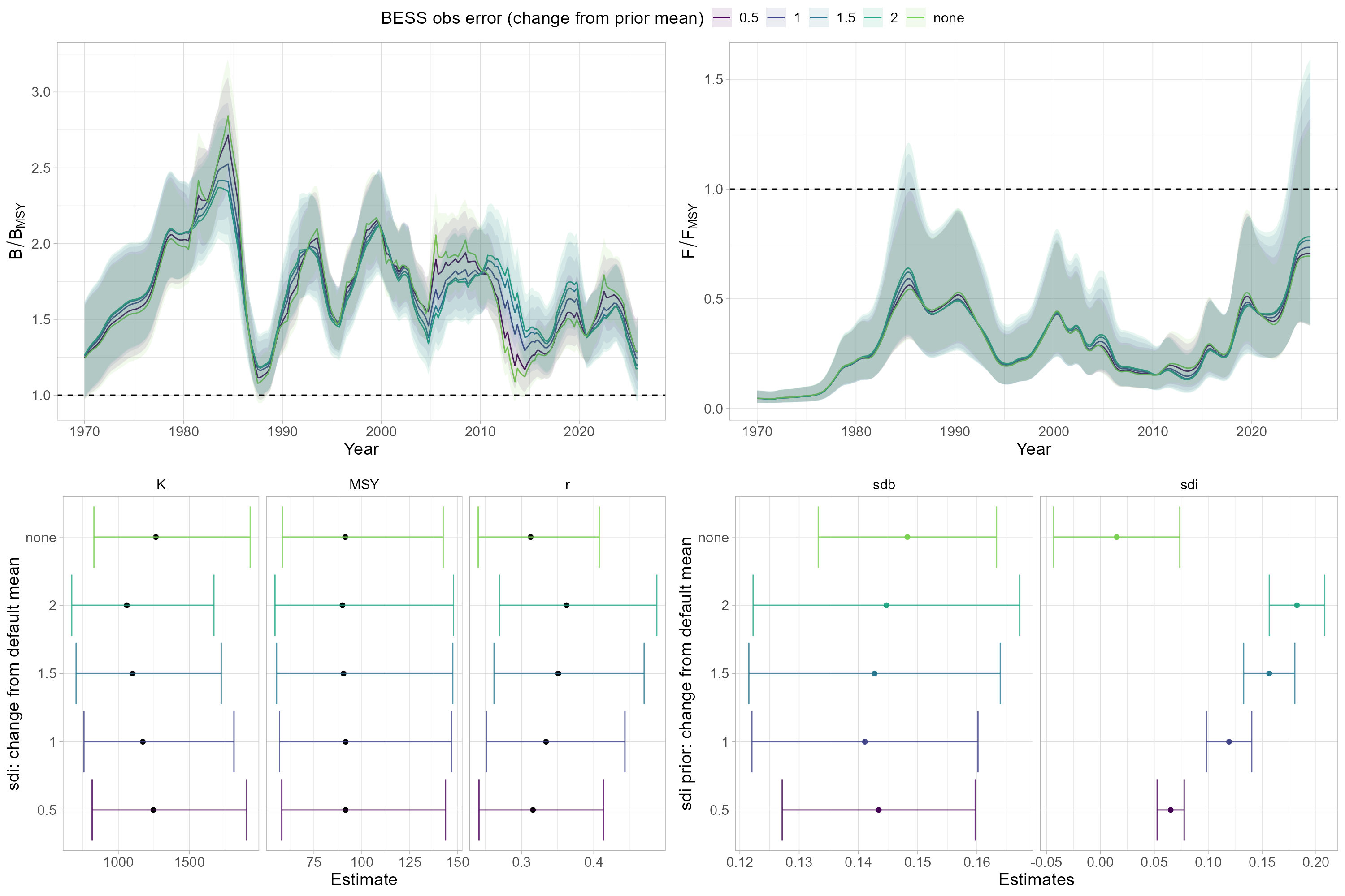
Figure 17: Sensitivity of model estimates of B/BMSY, F/FMSY, r, MSY and K, as well as biomass process error (sdb) and BESS index observation error (sdi) to the mean of the BESS sdi prior distribution. Included are model runs where BESS sdi prior mean was varied between 50 and 200% of the final model configuration, as well as a model run without a BESS sdi prior (“none”). Shown are esti-mated means (lines/dots) and 95% confidence intervals (shaded areas/error bars).
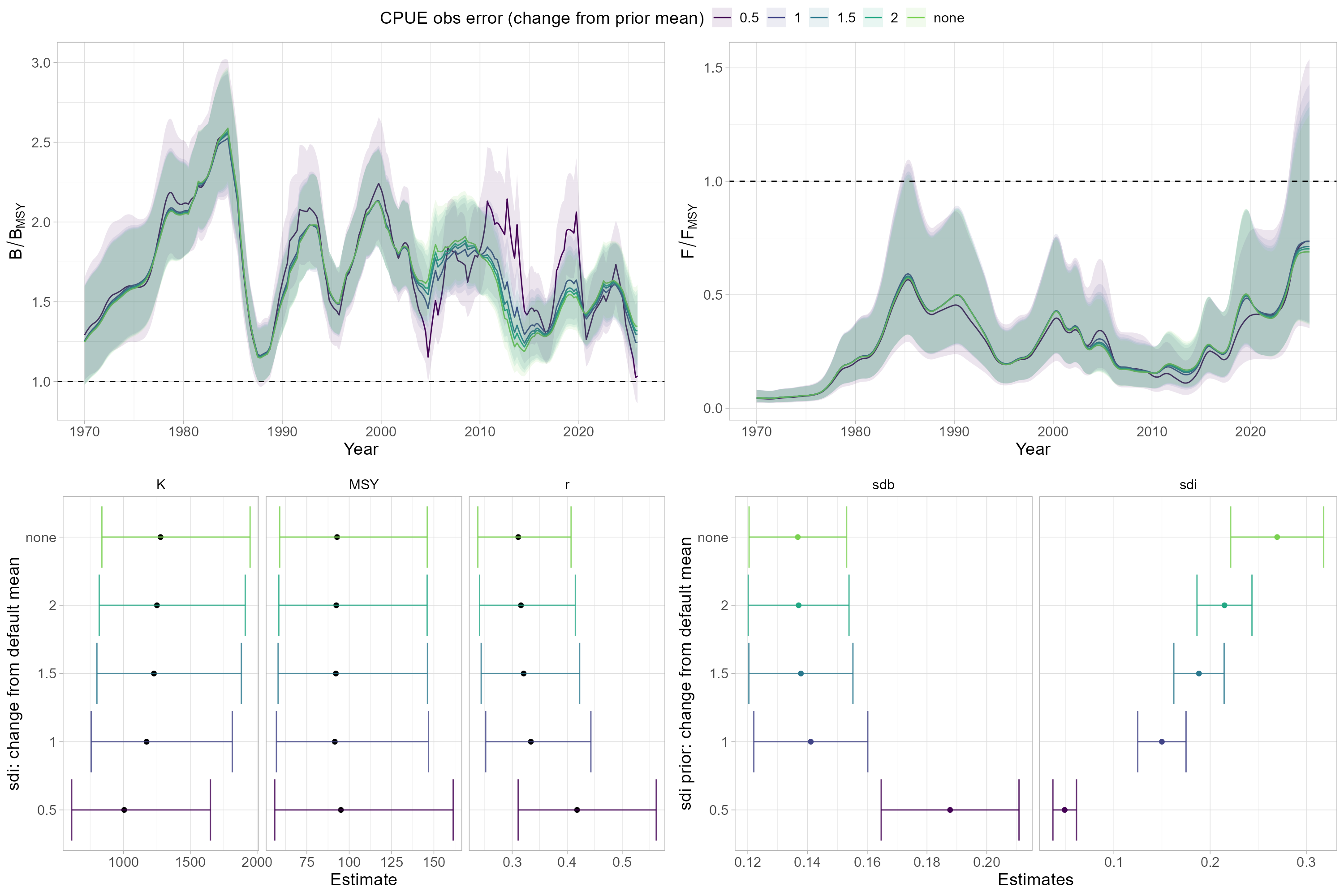
Figure 18: Sensitivity of model estimates of B/BMSY, F/FMSY, r, MSY and K, as well as biomass process error (sdb) and CPUE index observation error (sdi) to the mean of the CPUE sdi prior distribution. Included are model runs where CPUE sdi prior mean was varied between 50 and 200% of the final model configuration, as well as a model run without a CPUE sdi prior (“none”). Shown are estimated means (lines/dots) and 95% confidence intervals (shaded areas/error bars).
7.3 - Stock estimates
Relative exploitable biomass
Relativ fishing mortality
Year
B/BMSY (low)
B/BMSY
B/BMSY (high)
Catch
Predicted catch
F/FMSY (low)
F/FMSY
F/FMSY (high)
1970
0.87
1.42
2.29
6
5
0.01
0.04
0.12
1971
0.93
1.48
2.34
5
6
0.01
0.04
0.12
1972
1.00
1.55
2.42
7
6
0.01
0.04
0.13
1973
1.06
1.62
2.48
7
7
0.02
0.05
0.14
1974
1.10
1.66
2.50
8
8
0.02
0.05
0.15
1975
1.13
1.67
2.48
8
9
0.02
0.06
0.17
1976
1.16
1.69
2.47
10
11
0.02
0.07
0.21
1977
1.28
1.82
2.58
20
19
0.04
0.11
0.33
1978
1.46
2.03
2.83
39
33
0.06
0.17
0.51
1979
1.54
2.10
2.87
36
38
0.06
0.20
0.60
1980
1.56
2.08
2.77
46
43
0.07
0.22
0.69
1981
1.63
2.15
2.84
44
49
0.08
0.24
0.74
1982
1.70
2.25
2.97
63
65
0.10
0.30
0.95
1983
1.80
2.39
3.16
105
97
0.13
0.42
1.33
1984
1.87
2.51
3.36
128
122
0.17
0.53
1.71
1985
1.71
2.32
3.15
124
111
0.17
0.57
1.90
1986
1.28
1.75
2.38
65
69
0.15
0.49
1.64
1987
0.96
1.30
1.77
43
48
0.13
0.43
1.41
1988
0.87
1.17
1.59
49
49
0.14
0.44
1.41
1989
0.95
1.28
1.73
63
61
0.15
0.47
1.50
1990
1.14
1.54
2.08
81
74
0.15
0.49
1.56
1991
1.29
1.76
2.39
75
74
0.14
0.44
1.40
1992
1.42
1.93
2.62
69
67
0.11
0.37
1.19
1993
1.46
1.98
2.70
56
52
0.09
0.29
0.95
1994
1.33
1.80
2.44
28
33
0.06
0.21
0.69
1995
1.14
1.54
2.07
25
27
0.06
0.20
0.63
1996
1.15
1.55
2.08
35
33
0.07
0.21
0.69
1997
1.29
1.74
2.33
36
39
0.07
0.23
0.74
1998
1.45
1.94
2.60
56
55
0.09
0.29
0.93
1999
1.56
2.09
2.79
76
73
0.12
0.37
1.19
2000
1.56
2.10
2.84
81
77
0.13
0.41
1.32
2001
1.41
1.90
2.57
57
60
0.11
0.35
1.13
2002
1.35
1.82
2.46
61
58
0.11
0.34
1.11
2003
1.28
1.74
2.36
39
42
0.09
0.28
0.89
2004
1.15
1.56
2.12
43
42
0.09
0.30
0.95
2005
1.14
1.55
2.11
43
41
0.08
0.27
0.87
2006
1.23
1.67
2.26
30
31
0.06
0.19
0.62
2007
1.33
1.79
2.40
30
30
0.06
0.18
0.57
2008
1.35
1.81
2.44
28
28
0.05
0.17
0.54
2009
1.34
1.80
2.43
27
27
0.05
0.16
0.51
2010
1.34
1.80
2.42
25
26
0.05
0.15
0.50
2011
1.35
1.83
2.48
30
29
0.05
0.18
0.57
2012
1.25
1.71
2.33
25
25
0.05
0.16
0.53
2013
1.12
1.55
2.14
19
20
0.05
0.15
0.48
2014
1.02
1.40
1.93
21
22
0.05
0.18
0.56
2015
0.99
1.34
1.82
34
32
0.08
0.25
0.82
2016
1.00
1.36
1.84
31
31
0.08
0.25
0.80
2017
0.99
1.33
1.80
30
32
0.08
0.25
0.79
2018
1.12
1.51
2.04
56
55
0.12
0.37
1.19
2019
1.20
1.64
2.24
74
71
0.15
0.47
1.52
2020
1.15
1.57
2.14
58
59
0.14
0.44
1.41
2021
1.05
1.42
1.91
55
56
0.13
0.41
1.32
2022
1.12
1.51
2.04
60
61
0.13
0.42
1.35
2023
1.17
1.58
2.13
74
75
0.16
0.51
1.63
2024
1.18
1.60
2.17
95
90
0.20
0.64
2.10
2025
1.01
1.39
1.91
71
72
0.18
0.60
2.00
2026
0.86
1.24
1.80
Table 7: Shrimp in the Barents Sea. Estimated exploitable biomass, catch and fishing mortality over time. Exploitable biomass og fishing mortality are relative to BMSY and FMSY, with 95% confidence intervals (low and high values). Predicted catches are mean estimates of catches in the stock assessment model. Catch in the final year is based on preliminary information.