Report series:
Toktrapport 2026-23ISSN: 1503-6294Published: 18.11.2026 Cruise no.: 2026204003Project No.: 15662 Research group(s):
Akustikk og observasjonsmetodikk,
FiskeriProgram:
Marine prosesser og menneskelig påvirkning
Research group leader(s):
Rolf Korneliussen (Akustikk og observasjonsmetodikk) og Guldborg Søvik (Fiskeri)
Approved by:
Research Director(s):
Geir Huse
Program leader(s):
Frode Vikebø
Akustisk deteksjon og identifikasjon av makrell i nordsjøsildefisket
M/S Eros 27.5 - 6.6.2026
Makrell er en uønsket bifangstart i sildefisket i Nordsjøen. Markedsverdien under dette fisket er om lag 50 % av verdien i den ordinære makrellsesongen.
Dette toktet er en del av CRIMAC SFI og målet var å samle inn bredbånds- og smalbånds akustiske data for å utvikle metoder for bedre deteksjon av makrell under sildefisket i Nordsjøen. Arbeidet omfattet utvikling av metoder for innsamling av høykvalitets bredbånds akustiske data under kommersielt fiske, der flere instrumenter er i bruk og kan forstyrre ekkoloddet. Dataene ble analysert ved hjelp av eksisterende artsidentifikasjons‑algoritmer i LSSS Korona modul.
Resultatene viser hvor viktig det er å synkronisere og justere innstillingene på ekkoloddet for å minimere forstyrrelser fra andre instrumenter. Støyfjernings‑funksjonalitet i LSSS Korona modul kan brukes til å redusere støy som ikke kan fjernes ved synkronisering og justering av innstillingene. Artsdeteksjons‑algoritmen i Korona ser ut til å detektere de svake makrellmålene, men det gjenstår å fastslå om deteksjonen er tilstrekkelig presis, og hvilke frekvenser og om bredbånd kreves for tilfredsstillende deteksjon. Når dette er etablert, er neste steg å implementere metodene i praktiske verktøy for fiskeflåten.
Summary
Mackerel is an unwanted bycatch species in the North Sea herring fishery. Its market value during this fishery is about 50% of the value obtained in the main mackerel fishing season.
This survey is a part of the CRIMAC SFI and the objective was to collect broadband and narrowband acoustic data to develop methods for improved mackerel detection during the North Sea herring fishery. The work involved developing methods for collecting high-quality broadband acoustic data during commercial fishing operations, where several instruments are in use that may interfere with the echosounder. The data were analyzed using existing species-identification algorithms in LSSS Korona module.
The results show the importance of synchronizing and adjusting echosounder settings to minimize interference from other instruments. Noise-removal functionality in LSSS Korona module can be used to reduce noise that cannot be eliminated through synchronization and adjustment of the settings. The species-detection algorithm in Korona appears to detect the weak mackerel targets, but it remains to be determined whether the detection is sufficiently accurate and which frequencies and whether briadband are required for satisfactory detection. Once these have been established, the next step is to implement the methods into practical tools for the fishing fleet.
1 - Background
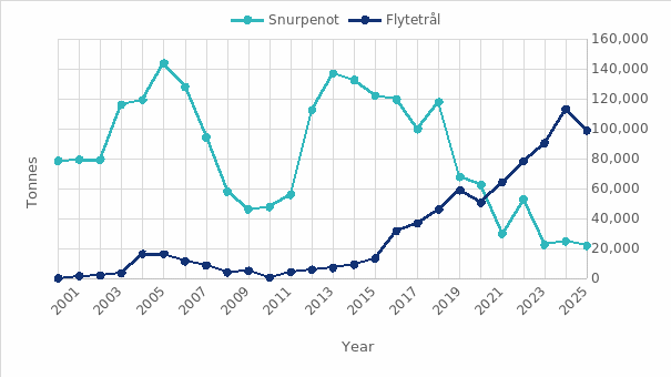
In May and June herring is fished in the Norwegian zone of the North Sea. The Norwegian quota in 2026 is 70 899 t, of which about 70% must be caught in the Norwegian zone (www.sildelaget.no). The boats use either purse seine or pelagic trawl to catch the herring. Both gears may be employed during a single fishing trip and the choice depends on the behaviour of the herring. If the herring are in distinct large schools purse seine is preferred, whereas pelagic trawls are preferred if herring are distriuted in scattered small schools. Many of the boats are equipped with steerable trawl doors that allow rapid adjustment of trawl depth from seabed to surface, depending on school location and several schools can be caught in one trawl haul. The use of pelagic trawl has increased since 2015 and has been the dominant gear since 2021 (Figure 1).
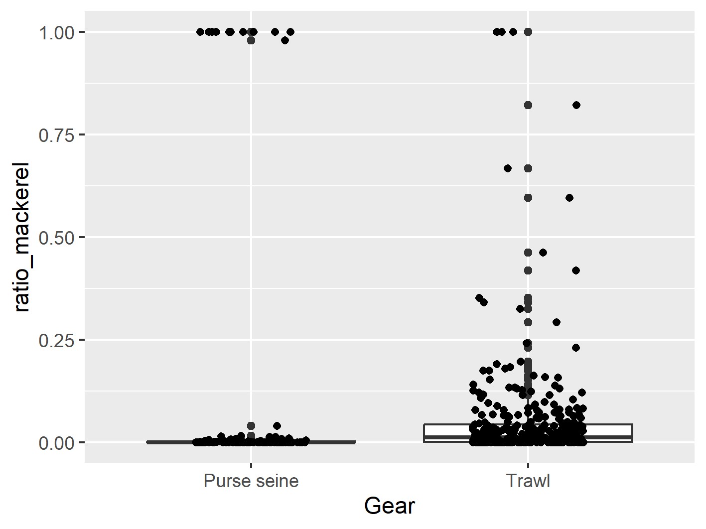
Mackerel is an unwanted by-catch in the fishery because the market price is about 50% of that in the main mackerel season. The mackerel are mainly distributed in small, low-density aggregations close to surface in the summer months (Nøttestad et al. 2015). This combined with the weak target strength makes mackerel difficult to detect with traditional acoustic methods. Bycatch risk is greater in trawls than in purse seines ( Figure 2 ), because trawl hauls can last several hours and sweep through a large area, whereas purse seines generally target and capture a single school.
Mackerel and herring have different acoustic frequency responses, and this can be used to distinguish between the species (Korneliussen et al., 2009). This approach is already in use in commercial fisheries (e.g. ES80 software) and scientific surveys (Korneliussen et al. 2016). Broadband acoustics provide higher vertical resolution and higher signal to noise ratio potentially improving mackerel distinction from background noise. CRIMAC has developed methods based on broadband echosounders to detect low density occurrences of mackerel. The methods were tested in the mackerel fishery on board Libas in 2021 with promising results. Information of individual fish size is also important for the fishermen. Small herring are used for fishmeal and oil giving lower prices and not an optimal strategi for providing high quality and sustainable seafood. While herring below 20 cm are illegal to catch. Size can be measured with acoustic methods (Kubilius et al., 2023 ), but these methods are not yet implemented into commercial fisheries. The methods also require detection of individual fish which may be challenging in high density schools.
The number of echo sounders and frequency bands needed to detect and identify mackerel should be reduced to the minimum, carefully assessing whether broadband is required or whether narrowband or shorter bandwidths can be used instead. Interference with other instruments used during fishing (e.g. fisheries sonars, ADCP, trawl sensors) that operate in the same frequency bands as the broadband echosounders (almost continuous from 18 to 380 kHz) will be a challenge. Synchronization between instruments is therefore required. Careful consideration of what is required is also important to avoid unnecessary expensive investments on the fishing boats.
CRIMAC partners IMR, Kongsberg Discovery and EROS AS aim to develop improved acoustic methods for species and size identification in North Sea herring fishery and that are practical to implement on fishing vessels. The objectives of the cruise were to:
Develop methods for collecting good quality (synchronized) broadband data on board fishing vessels
Collect acoustic and trawl data during the fishery
Based on the collected data and the characteristics of the fishery, develop recommendations for improving current methods for detecting mackerel (ES80/EK80), and propose new methods informed by the challenges observed during searching and fishing operations (e.g. Algorithm/Korona for live species identification).
Figure 1 . Proportion of North Sea herring caught with purse seine and trawl. Figure from Fisheries Directorate.
Figure 2 . Ratio of mackerel in purse seine and trawl catches in the North Sea herring fishery. Data from sale slips Fisheries Directorate
2 - Description of the capture process on board MS EROS
Search: The low frequency sonar (Simrad ST90) with 2500 m range is used for searching. Vessel speed is 9 – 10 knots.
School detection: When a school is detected a marker is placed on the school on the sonar display. The course is set toward the school. As the school moves, new markers can be placed on top of it to measure swimming speed and direction.
School evaluation: School size, position, swimming direction and speed are evaluated first with the low frequency sonar, and once at closer range with the medium frequency sonar (Simrad MF90 – 1000 m range). The vertical beams are used when the school is within 600 m. The Furuno high frequency sonar (FSV75) is used for more detailed evaluation of behaviour when within 600 m range. The SN90 inspection beams can give additional information on depth and density (~300 m range). The sonar ranges are adjusted depending on distance to school.
Selection of gear. The size of the school mainly determines whether trawl or purse seine is used. For medium to large schools purse seine is preferred. If several small or medium schools are in the area trawl is preferred.
Purse seine. Before setting the seine, the vessel usually circles the school one or several times to monitor swimming behaviour and determine the optimal setting of the seine. Since sailing over the school may affect the school behaviour, echosounders are rarely used during purse seining, except when there is uncertainty regarding species identification. All sonars are also used to keep track of the school while setting the purse seine. When the purse seine is pursed sonars on hull units need to be retracted to avoid damage.
Trawl. An overview of schools and their positions is first obtained with echosounders and sonars. The trawl is then set often turning back to cover the monitored area. Trawl depth is set based on the depth of school on the echosounder and some estimate of reactions to the vessel and trawl. Trawling can be on the seabed or close to surface. Trawling close to surface is, however, avoided due to higher risk of by-catch. The echosounders are also used to get an idea of species, and the depth of the trawl can be adjusted to try to avoid the school if a suspected wrong species is observed on the echosounder. Trawl sonar is used to confirm that schools enter the trawl and the trawl eye to confirm catches entering the codend. Catch sensors give an indication of total catch in the codend.
3 - Methods
3.1 - Installation of WBTs
The echosounder transducers on Eros are of types ES18-11, ES38-B, ES70-7C, ES120-7C, ES200-7C, and ES333-7C. The 18 and 38 kHz transducers can only be operated with narrowband pulses, commonly referred to as continuous wave (CW), whereas the remaining transducers support frequency modulated broadband (FM) pulses. Eros was originally equipped with one wideband transceiver (WBT). Additional WBT units for the remaining transducers were borrowed from IMR and installed on board by Kongsberg Discovery prior to the survey.
3.2 - Calibration of EK80
Prior to the calibration EK80 software was updated from version 1.12.4 (2019) to 25.2.3 (2025). Environmental parameters were also measured before the calibration with a RBR concerto3 CTD (serial number 204775) at 30 m depth, corresponding to the calibration sphere depth. The parameters were entered into the EK80 software prior to calibration: speed of sound 1477.5 m/s, temperature 7 ºC, conductivity 34.11 mS/cm, and salinity 33.7 ppt.
Both CW and FM settings were calibrated since we aimed to evaluate results both from narrowband and broadband. Broadband could be used from 50 – 380 kHz. The echo sounders were calibrated with tungsten carbide (WC) spheres with diameters of 57.2, 38.1, 35 and 25 mm, according to standard calibration procedures (Demer et al. 2015). The calibrated settings, and the calibration spheres used are given in Table 1 and Table 2 .
Two spheres (WC38.1 and WC35) were used for the broadband calibration of the 120 kHz transducer, three spheres (WC38.1, WC35 and WC25) were used for the 200 kHz transducer, and two spheres for the 333 kHz transducer (WC25 and WC22) because the frequency responses of individual spheres contain deep nulls that must be avoided during calibration. These nulls were excluded by defining stop bands in the EK80 software. When more than one sphere is used for a single transducer, EK80 merges the calibration results by prioritizing one sphere at each frequency step, so that the other sphere(s) provide data within the excluded frequency bands of the first sphere.
Chanel
Transducer type
Pulse shape
Bandwidth [kHz]
Taper
Pulse duration [ms]
Power [W]
CW (Continuous Wave)
18-CW
ES18-11
CW
-
Fast
1.024
800
38-CW
ES38-B
CW
-
Fast
1.024
400
70-CW
ES70-7C
CW
-
Fast
1.024
225
120-CW
ES120-7C
CW
-
Fast
1.024
100
200-CW
ES200-7C
CW
-
Fast
1.024
105
333-CW
ES333-7C
CW
-
Fast
1.024
40
FM (Frequency Modulated)
70-FM
ES70-7C
FM-Up
50-85
Fast
2.048
225
120-FM
ES120-7C
FM-Up
95-165
Fast
4.096
100
200-FM
ES200-7C
FM-Up
170-260
Fast
4.096
105
333-FM
ES333-7C
FM-Up
280-380
Fast
4.096
40
Table 1 : Overview over echo sounder settings.
18CW
38CW
70CW
70FM
120CW
120FM
200CW
200FM
333CW
333FM
Sphere ID
BW (kHz)
-
-
-
50-85
-
95-165
-
170-260
-
280-380
IMR104
WC57.2
X
X
IMR002
WC38.1
X
X
X
X
X
X
IMR123
WC35
X
X
IMR132
WC25
X
X
IMR071
WC22
X
X
Table 2 : Overview over calibration spheres used
3.3 - Synchronizing acoustic instruments
During the fisheries there are several instruments that transmit acoustic signals with frequencies overlapping with both the broadband and the narrowband echo sounders.
Instrument overview on Eros
ST90 MK2
Type: Low‑frequency 360° omnidirectional sona
Frequency:14 - 24 kHz
Range: typically 10 - 5000 m (up to 14000 m on display, range depends on conditions)
Beam: One horizontal and one vertical beam; up to 360º coverage in plane view with electronic tilt from -10 º to 90 º , (horizontal/inspection views -10 º to 60 º, vertical views 0 - 90º
MF90
Type: Medium-frequency 360° omnidirectional sonar with a cylindrical multi‑element transducer, electronic tilt.
Frequency: 75 - 85 kHz (selectable centre, 2 kHz bandwidth)
Range: 25 - 2000 m
Beam: One horizontal and one vertical beam; up to 360º coverage in plane view with electronic tilt from -10 º to 90 º , (horizontal/inspection views of -10 º to 60 º , vertical views 0 º to 90 º ).
SN90 (with LPT32 transceiver board)
Type: Sonar with two fans (one vertical, one sideways) + 5 beams
Frequency: 70 - 120 kHz
Range: 25 - 2000 m
Beam: Fan horizontally 120º or -80 to +80º; vertically -40 to +40º (inspection beams -80 to +80º)
FSV75
Type: Furuno half‑circle sonar with fast sweep
Frequency: 180 kHz
Range: 50 - 2000 m
Beam: Half‑circle beam 180º in 8 s, tilt 0 - 90º, train -175 to + 175º
ES150‑3C
Type: ADCP with 4 beams, can be used as a narrow‑beam echosounder
Frequency: centre 150 kHz (130 - 170 kHz)
Range: On the order of a few hundred metres
Beam: Four narrow beams, about 3º beamwidth, 30º tilt
Catch and gear monitoring and steering systems
The Multi Level Door, MLD trawl steering system uses broadband signals for communication between the doors and the boat in the frequency range 7-17 kHz.
Trawl catch sensor (Marport): uplink frequency 41 – 45 kHz
Trawl door sensors (Marport): uplink frequency 41-43 kHz
The distance from the ship to the echo sounder and sonar in the trawl is about 400 -600 m. It is therefore unlikely that trawl sensors disturb the ship mounted echo sounders directly. However, sensors communicate and transmit data to a receiver on the vessel as acoustic communication signals, which may cause some interference at 38 kHz. Since we used narrowband operation, the system is less sensitive to such interference. The uplink frequency is the acoustic communication frequency used by the trawl sensors to transmit data to the vessel’s receiver.
Syncronization software
The Simrad TU40 trigger system consists of a trigger unit and control software that synchronize multiple acoustic instruments. The instruments are physically connected to the trigger unit. In the TU40 software, which runs on the EK80 PC, the EK80 system is defined as the reference, and all other equipment must adapt their pinging frequency to it. The purpose is to prevent disturbing signals from other acoustic systems from being received by EK80. In addition to setting EK80 as the reference system in the TU40 Runtime settings menu the EK80 must also be defined as the master in the EK80 software. This is defined in the EK80 software installation menu, under synchronization. The other instruments should be configured as slaves in their installation menu in their respective softwares, and in the TU40 software the “reference system” button for these instruments should be set to “off”.
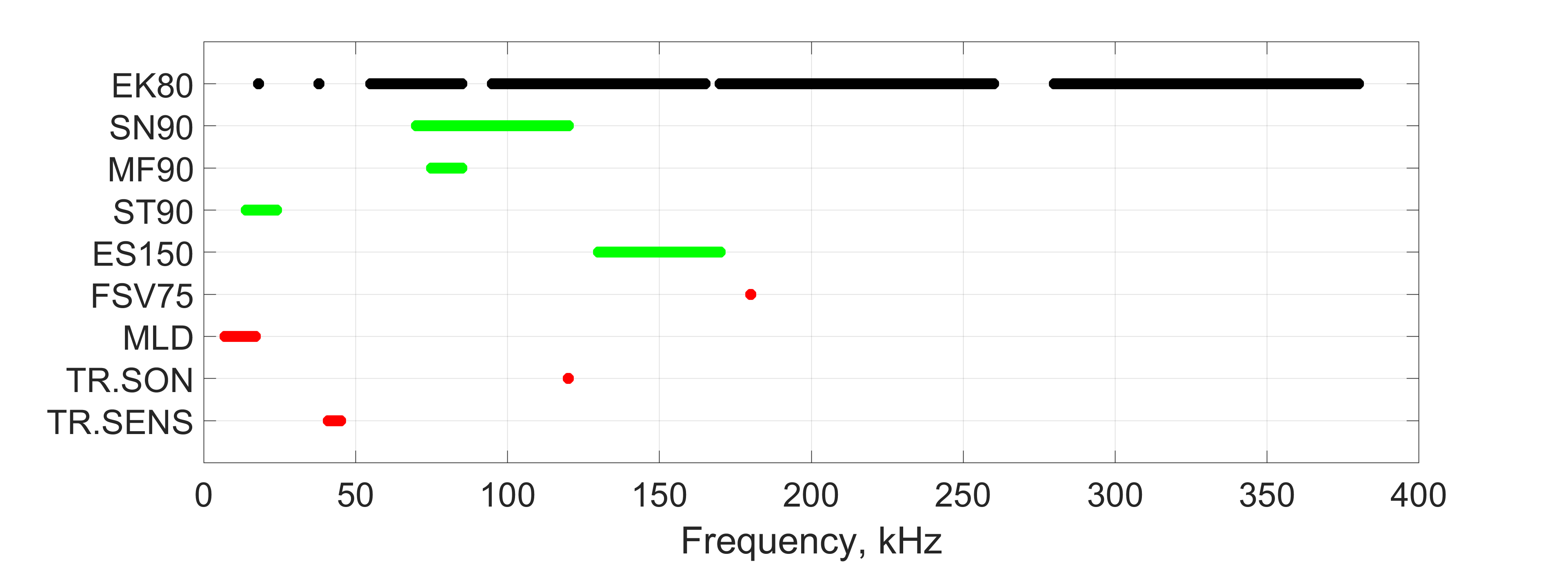
The trigger unit controls the instruments with a “ready to transmit” signal. If the delay is set to zero, all connected instruments transmit simultaneously. The instruments that can be synchronized with TU40 are SN90, MF90, ST90 and ES150. Instruments that cannot be synchronized include the 180 kHz Furuno sonar FSV75, and all acoustic communication systems between boat and trawl related to the trawling operations, see overview in Figure 3 .
Figure 3 : Overview over the frequency bands used by different instruments. EK80 is set as the master, and the instruments in green are synchronized with EK80. The instruments marked in red are not possible to synchronize. TR.SON is the trawl sonar, and TR.SENS are the trawl sensors for doors and catch.
When synchronizing, the goal is to ensure that signals from other systems are transmitted only after EK80 has completed its transmit–receive cycle. The required delay can be approximated by the two‑way travel time to the seabed, i.e. t=2*depth/c, where c is the sound speed. For a depth of 125 m and c=1490 m/s, this gives a delay of 250/1490=0,167 s (167 ms). This represents the minimum delay for this depth since the fishermen need to see the bottom on the echo sounders when trawling on or close to seabed.
3.4 - Data collection and analyses
Acoustic data were continuously collected on the fishing grounds during searching and capture. The echosounders were manually altered between FM and CW. Initially the aim was to automatically alternate pinging but it was difficult to set up and we considered it to be impractical as the ping interval needed to be adjusted as fishing conditions changed to maintain optimal synchronization.
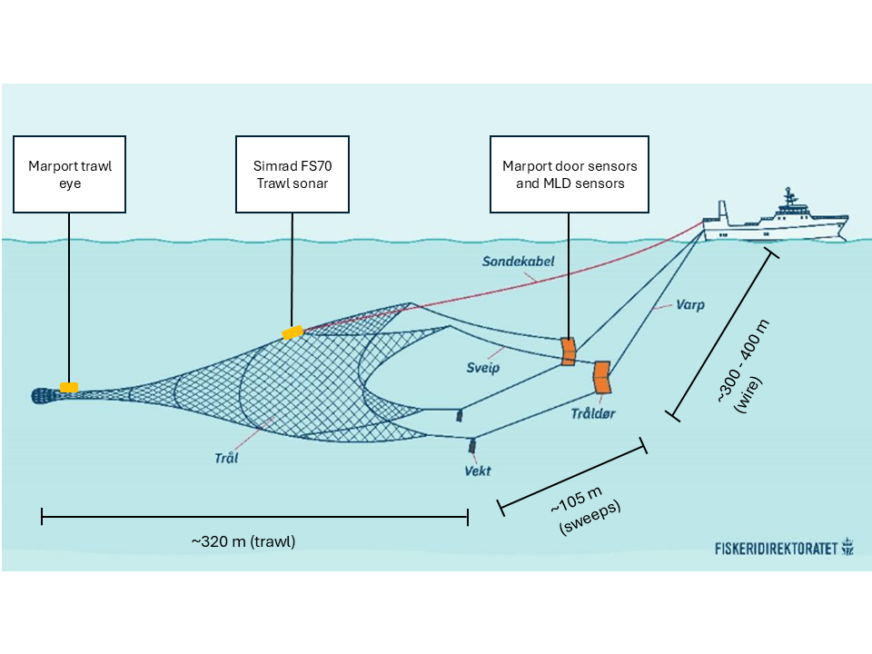
Catch start and end times and positions were registered. During trawling boat speed, length of trawl wire, door depth and spread were logged ( Figure 4 ). Schools that were captured (registered on trawl sonar and trawl eye) were also noted down. In trawl haul 5 a GO PRO was mounted ahead of the codend in the side panel looking horizontally into the trawl.
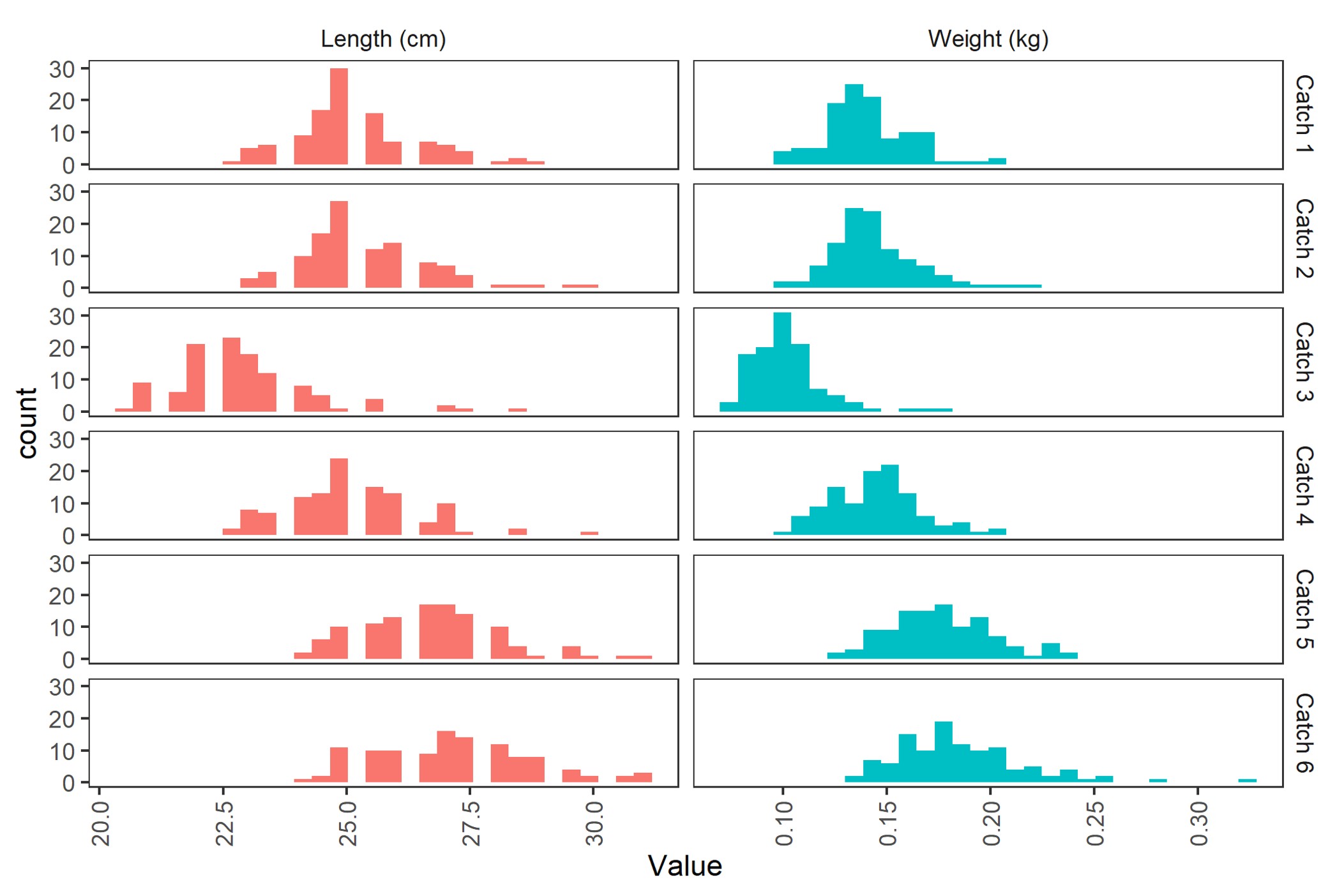
Total catch quantity by species and weight distributions were obtained from the official catch logs. As the catch is pumped on board, the crew collect continuous samples of individual fish weights. From these samples we measured the weight and length of 100 herring and all mackerel in the samples.
Three CTD casts were made at the fishing grounds. The number of casts and the depth were limited by the risk of getting the CTD line into the propellers.
For comparisons of detections with the vessel echosounder and with trawl catches the time difference for passing the same spot was calculated by the following equations:
x = √((wire length + sweep length)2 - depth2)
v = (hauling speed in knots * 1.852 m/h) / 3600
t = x/v
Where x is the horizontal distance between the boat and the trawl opening, depth is the depth of the trawl. v is the vessel speed in meters pr. second and t is the time difference between spotting the school on the echogram until the same school enters the trawl.
Figure 4 . Illustration of a pelagic trawl (Fiskeridirektoratet) with the length of the trawl, sweeps and wire and the position of the main sensors.
3.5 - Echosounder data analyses: Sv(f) and species identification in Korona LSSS
Echosounder data were analysed with the software Large Scale Survey System (LSSS) (Korneliussen et al. 2018) and Korona (a module in LSSS).
While working with the Eros data, the detection of schools was not working optimally. New functionality was introduced into LSSS that seemed to overcome the shortcomings. The functionality will be incorporated in the January 2027 LSSS version after extensive testing, but until then the new school-detection functionality is only available to the developers of LSSS.
During the cruise, before we had the updated school detection functionality, we investigated the frequency dependence of Sv for the schools by using LSSS version 3.2.0. For each school that was caught we plotted the Sv(f) and also Sv(f) relative to 38 kHz to see if we were able to see any obvious features in the frequency response by eye. We do not have enough data to investigate this statistically, but still we tried to compare the frequency response from catches with different fish lengths to look for any size variation We also made a detailed scrutiny of the upper 50 m to look for individual or small aggregations of mackerel.
4 - Results
4.1 - Calibration
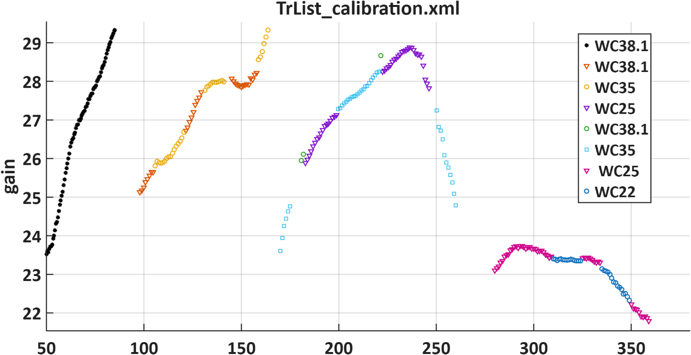
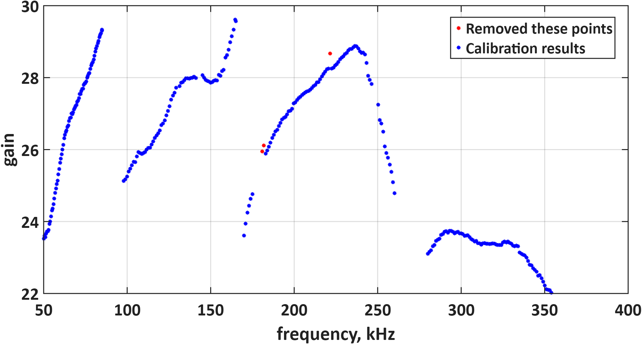
When calibration data from more than one sphere is available within the same frequency range, the EK80 software merges the results by selecting one sphere at each frequency step. In this way, each frequency step is calibrated using data from a single sphere only. Inspection of the broadband gain curves showed that the 200 kHz calibration contained a few clear outliers, all associated with the WC38.1 calibration sphere. In contrast, calibrations using the smaller spheres, WC35 and WC25, produced smoother and more continuous gain curves. The original gain curves are shown in Figure 5 , and Figure 6 presents the curves after manual removal of the outliers.
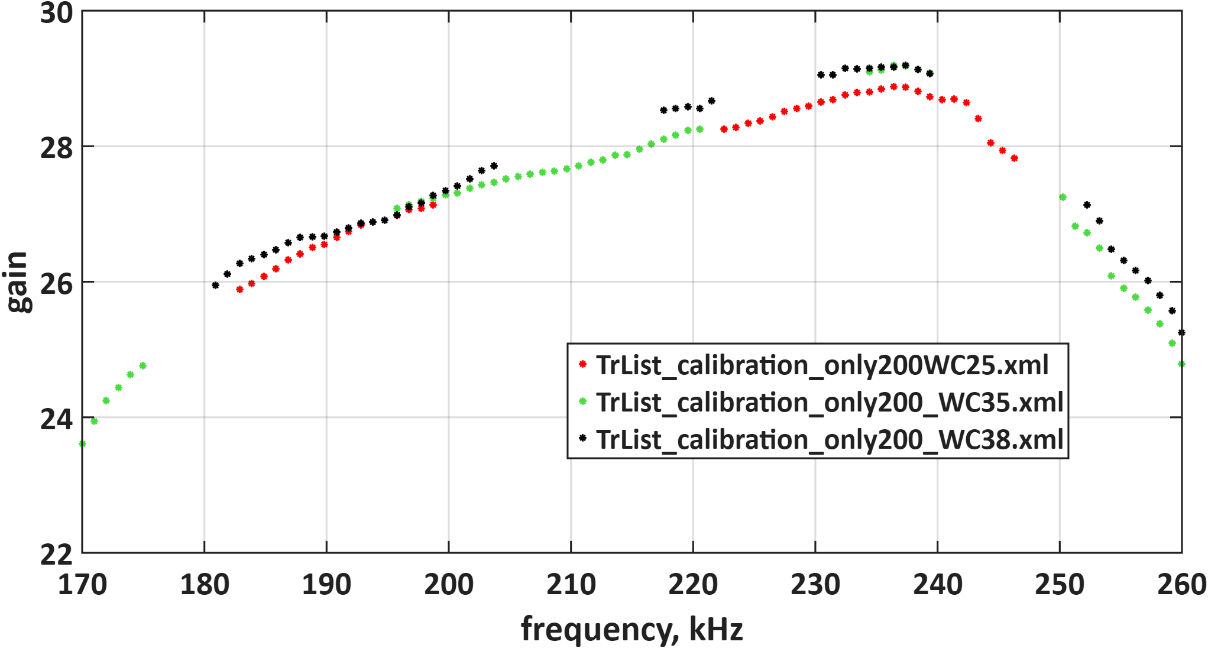
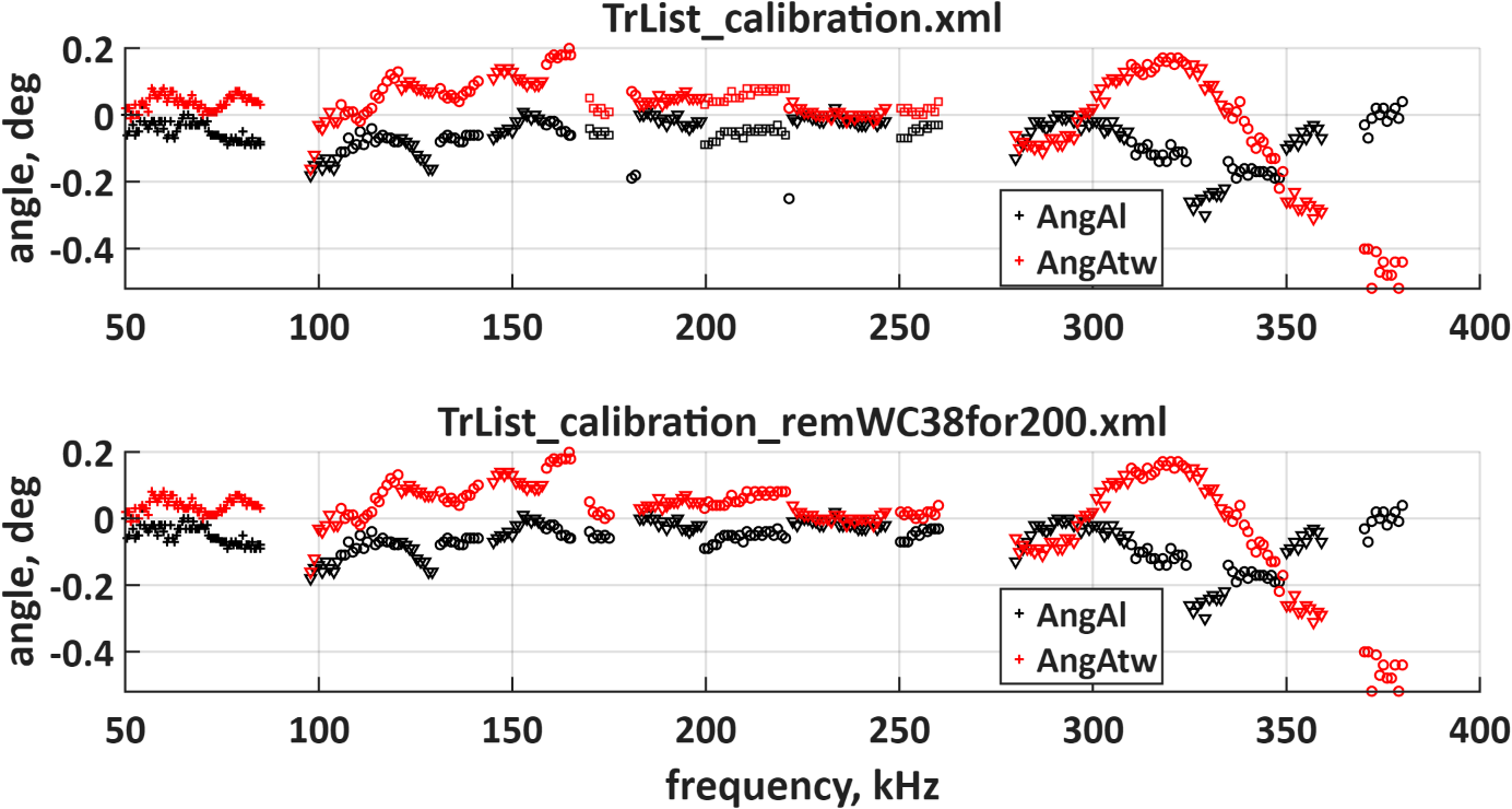
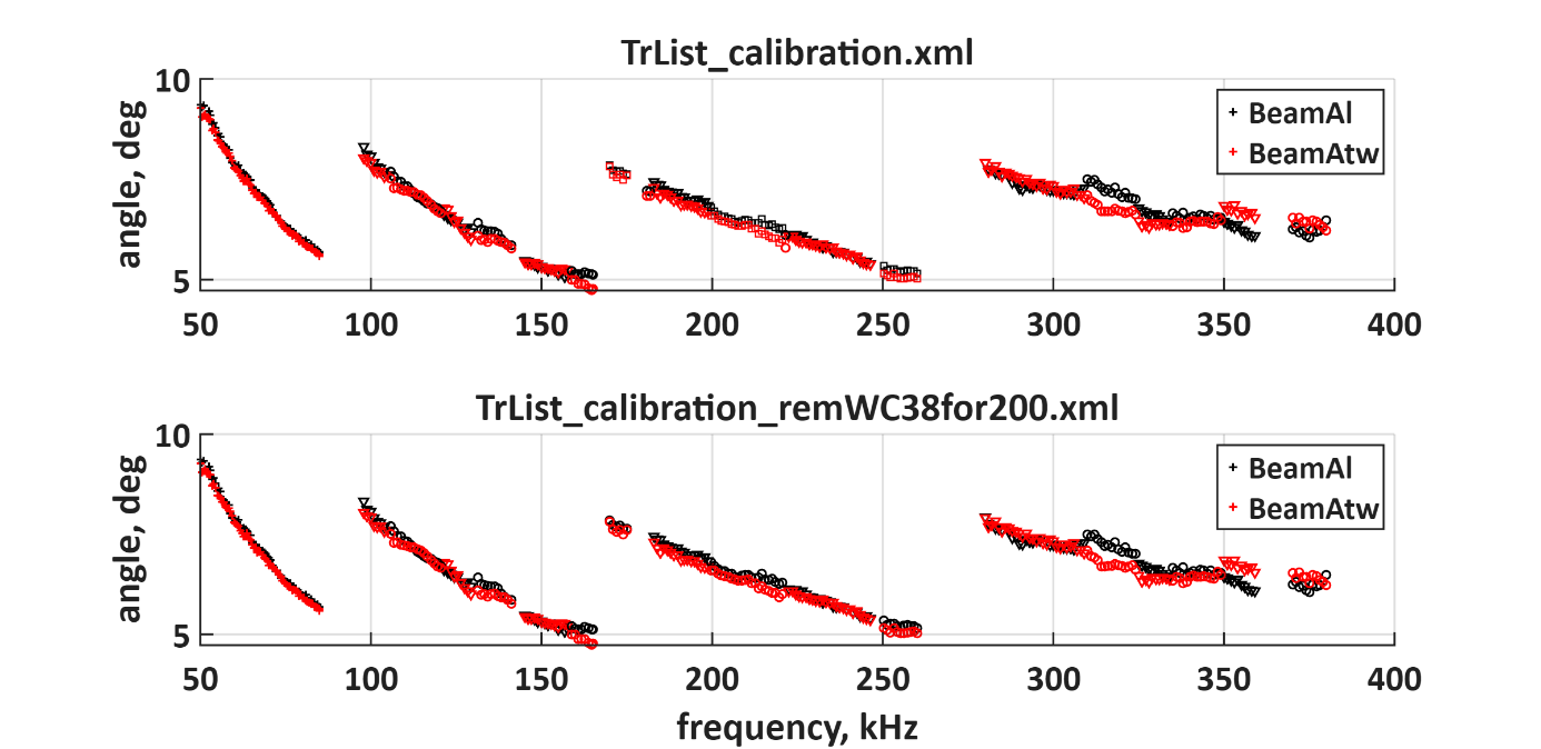
The calibration gains obtained with the three spheres at 200 kHz were then compared ( Figure 7 ). Although some differences among spheres are evident, WC25 and WC35 provided the most consistent results. The WC38.1 calibration data also appeared as outliers in the alongship angle offset ( Figure 8 ), but this effect is not clearly visible in the beamwidth estimates ( Figure 9 ).
Figure 5 : Calibration gain. Original calibration results before removing outliers
Figure 6 : Removing outliers (all results from WC38.1) from the gain curves
Figure 7 : Comparing calibration gain for 200 kHz for three different calibration spheres
Figure 8 : Angle offsets alongship and atwartship. The upper panel is before removing outliers, the lower panel is after.
Figure 9 : Bandwidth alongship and atwartship. Here the outliers are not as visible. Upper panel is before removing outliers, the lower panel is after.
4.2 - Synchronization
When synchronizing multiple acoustic instruments, the ping interval of the reference system (EK80) is a critical parameter, as it will influence both the ping interval and the transmission delay of the other instruments.
To detect loose aggregations of mackerel, the EK80 ping rate should be as high as possible. At the same time, the fishermen, in most cases, need to see the bottom (this was not needed in the last part of the cruise while we were trawling in the upper water layer). To avoid noise from a “false bottom” caused by bottom echoes from the previous ping at 150 m depth, the ping interval must be larger than 2*150/1490=0.200 s (200 ms) so that the previous bottom reflection has returned before the next ping is transmitted. In practice, the shortest ping interval that EK80 could achieve in FM mode when logging to 150 m depth was about 330 ms.
Several of the sonars also have vertical beams that produce bottom echoes. If these signals are delayed by approximately 200 ms relative to the EK80 bottom reflection, they further constrain the maximum ping rate. In that case, the ping interval must be increased to at least 400 ms to avoid interference from bottom echoes generated by the other sonars.
A ping interval of 350 ms was tested, and at greater depths (around 350 m) it was possible to remove interference from all synchronized systems. However, at shallower depths typical of the fishing grounds, a longer ping interval of about 500 ms was required to eliminate the noise.
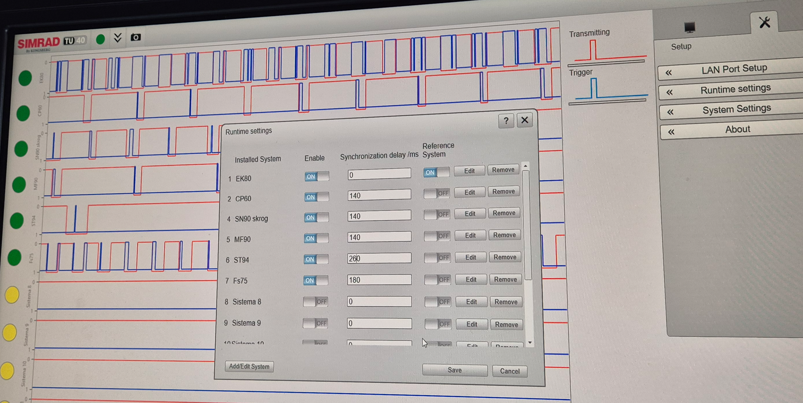
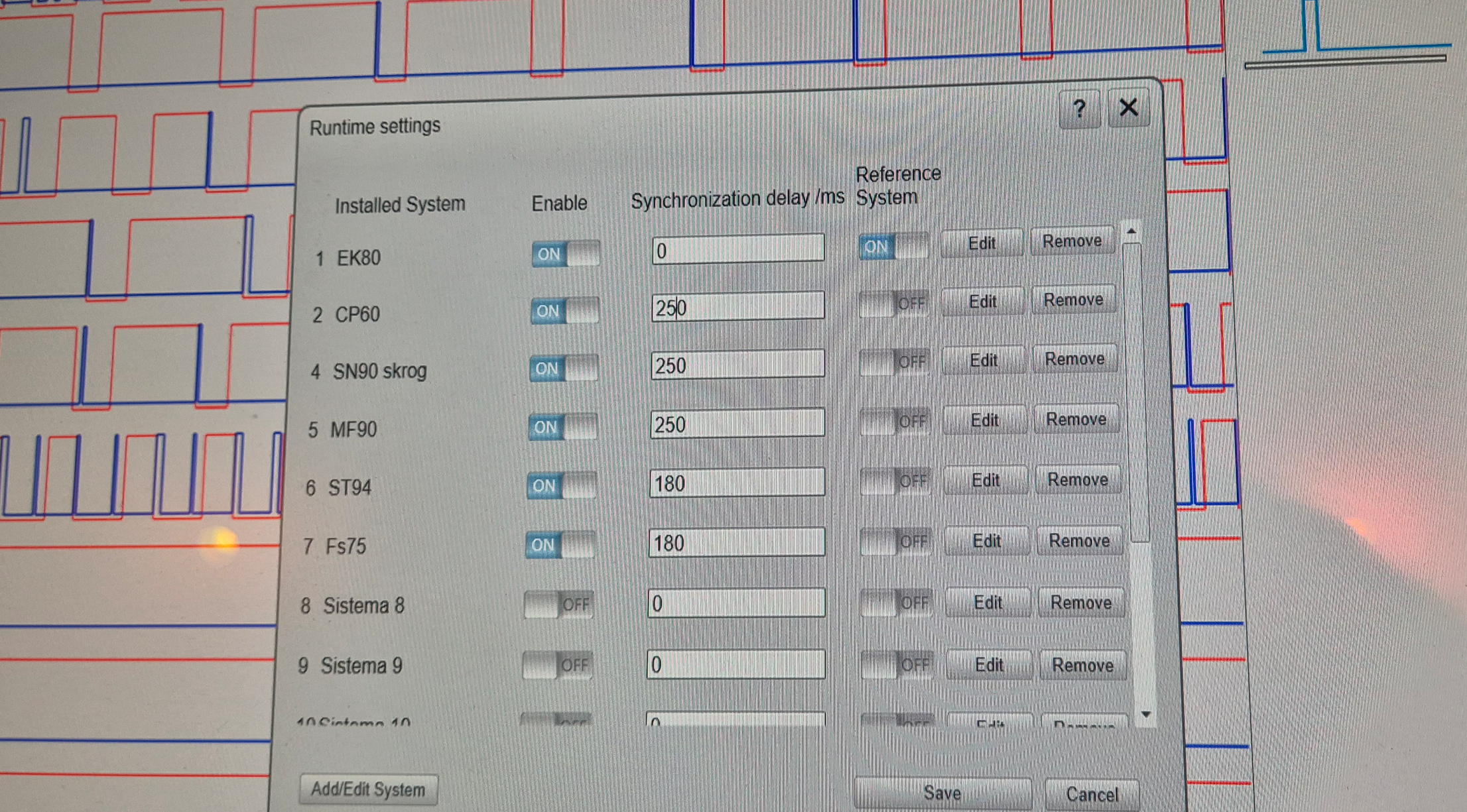
The settings of TU40 were adjusted several times during the survey depending on bottom depth and sonar settings. The ADCP noise seemed to shift with time by itself. The tilt and range of the sonars were often changed by the fishermen while searching for fish. EK80 had 0 delay, while the other instruments had a delay between 140 and 300 ms depending on the current situation with a pulse interval of about 500 ms. Examples of settings on TU40 are shown in Figure 10 and Figure 11 .
Interference on EK80 is most pronounced in broadband mode but is also evident in narrowband. The 18 kHz transducer, which can only be operated with CW pulses, is the noisiest channel, mainly due to the ST90 MK2 sonar and, during trawling, the MLD trawl door system. The ST90 MK2 uses long, low-frequency pulses with both a vertical beam and a horizontal fan, generating substantial noise across most of the 18 kHz detection zone for any TU40 setting. Adjusting the ST90 vertical beam frequency from 16 to 22 kHz removed interference from the vertical beam, leaving only the 16 kHz horizontal beams. Synchronizing these remaining beams with EK80 was possible, but difficult and very sensitive to changes of the sonar settings which was frequently done by the fishermen. In some cases, small adjustments to the EK80 pulse interval further mitigated interference.
180 kHz signals from the Furuno FSV75 sonar were interfering with the 200 kHz transducer in FM mode. This sonar could not be synchronized by TU40, at least it was not known how to. FSV75 was connected to the TU40 trigger box, and it was on the list of equipment in the software, but the problem was that it could not be defined as a slave in its own software. The solution was to adjust the bandwidth of the 200 kHz EK80 echo sounder from 170-260 to 190 to 260 kHz so it did not detect the signals from the FSV75 sonar.
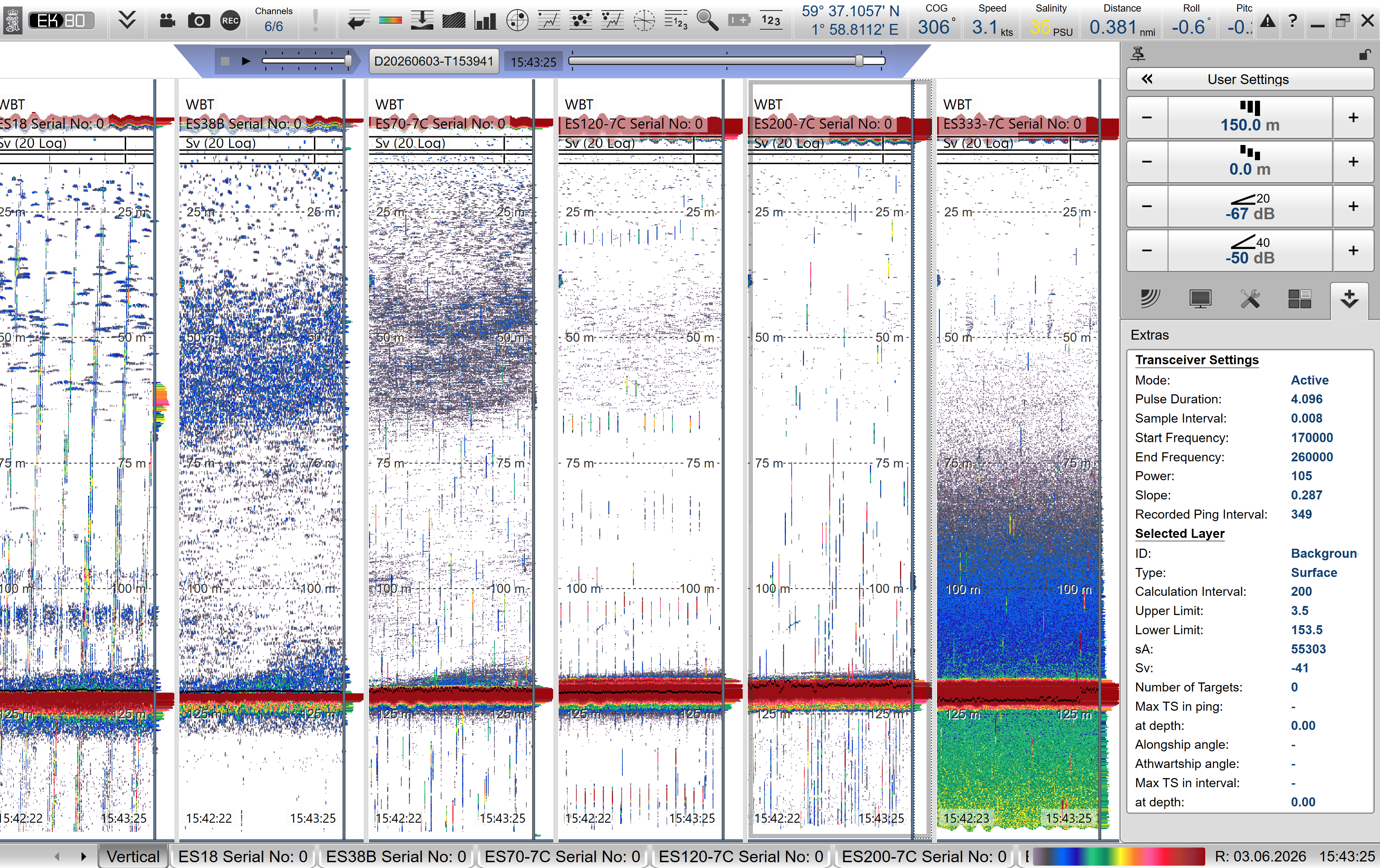
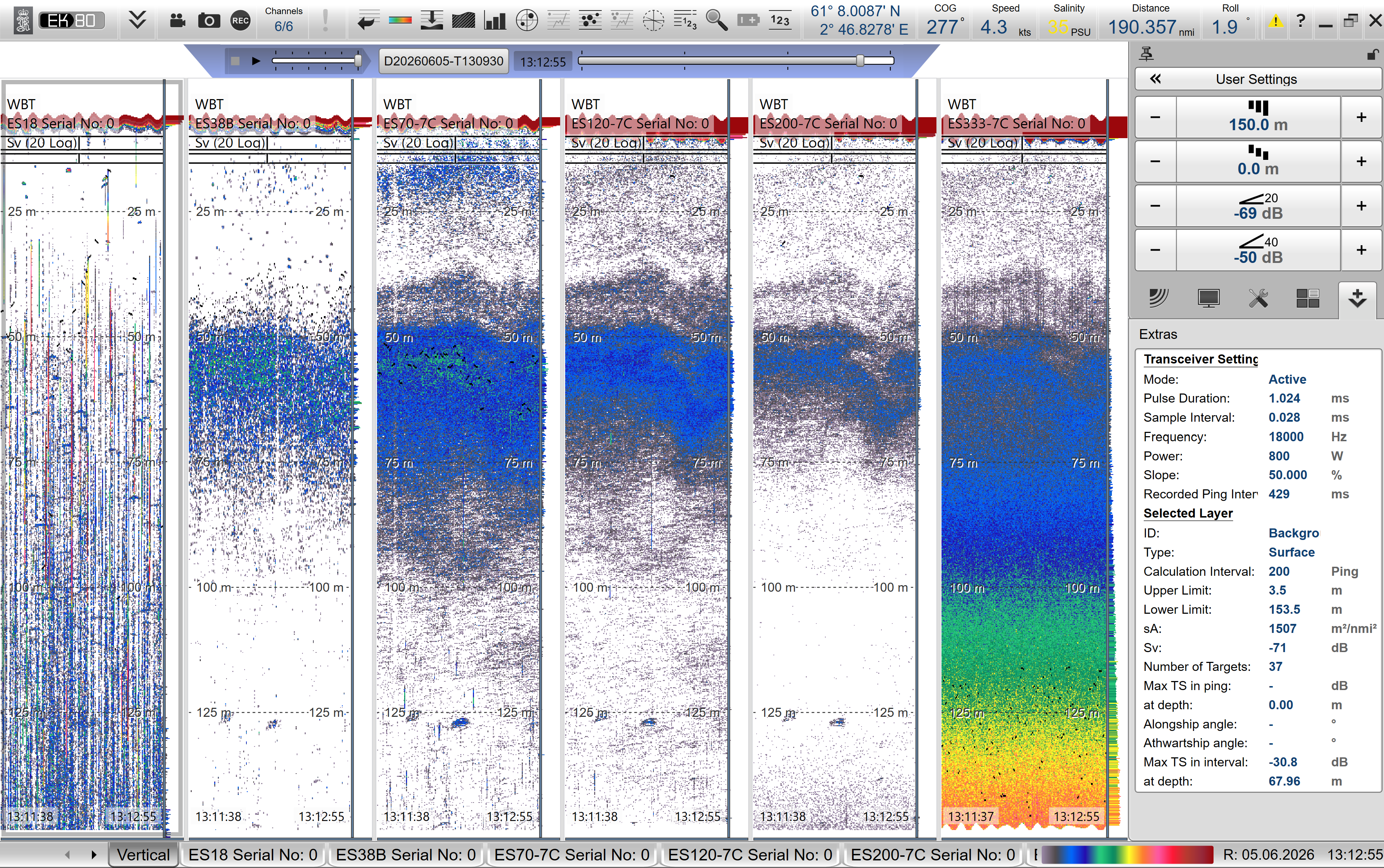
Example of noise before and after synchronizing the instruments are shown as before in Figure 12 and after in Figure 13 . Example of noise after synchronization, but during trawling are shown in Figure 14 .
Figure 10 : TU40 settings for CW measurements 5. June at 112 m depth and 500 ms ping interval
Figure 11 : TU40 settings used for FM measurements 4. June at 125 m depth and 500 ms ping interval
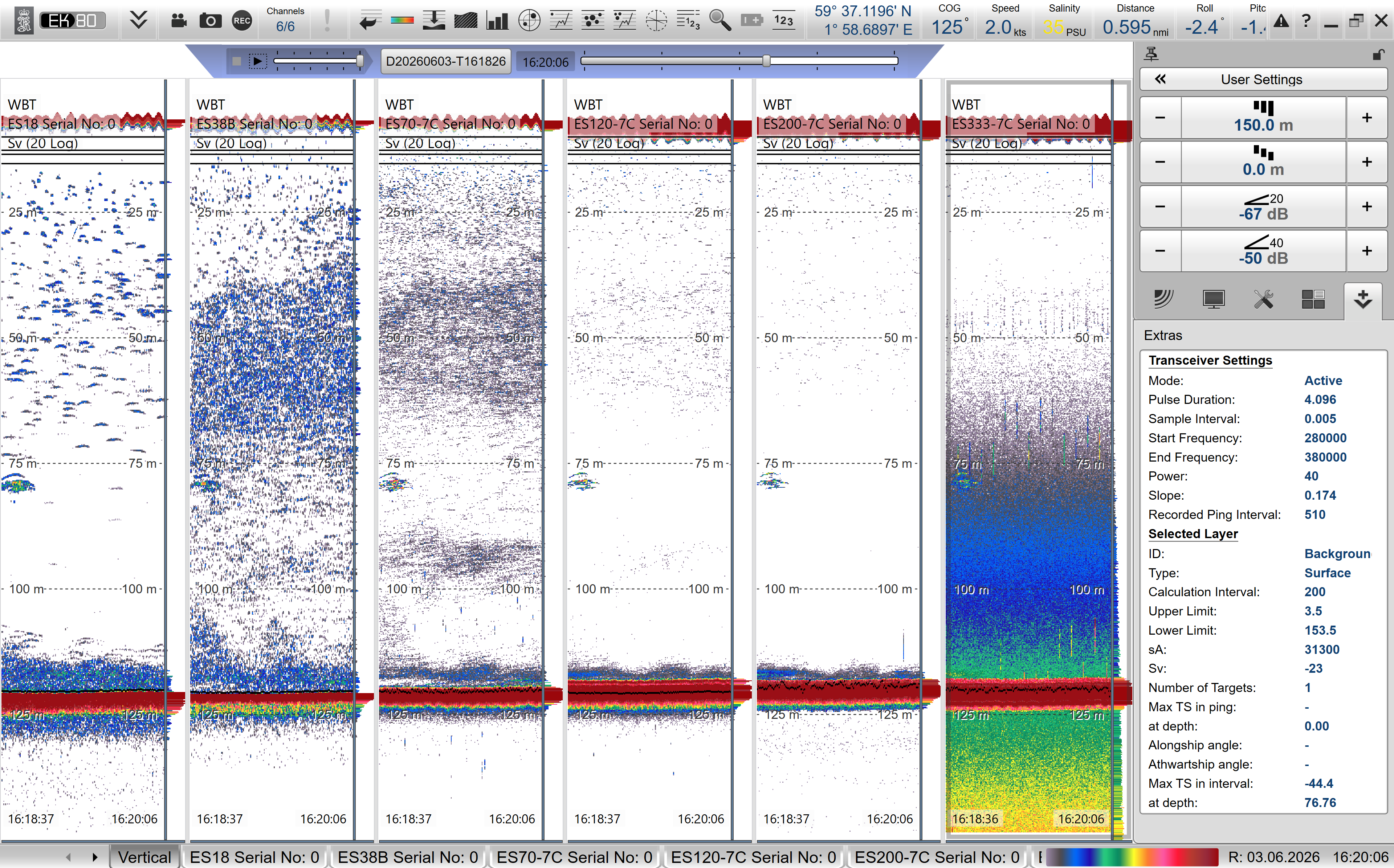
Figure 12 : Without synchronization. All acoustic equipment on. 350 ms ping interval. 200 kHz in full bandwidht. (38 kHz is quite clean, but they have turned off their other 38 kHz echo sounder for this survey).
Figure 13 : With synchronization. 500 ms ping interval. 200 kHz in reduced bandwidth. Still a little bit of noise here and there, but much better. (Notice that ping interval changes with about +/- 10 even if it is set to 500.
Figure 14 : Noise during trawling. The 18 kHz is affected by noise from the MLD (multi level door system for trawl) that can not be synchronized. Some other noise is seen, probably originating from the sonars that the fishermen adjust during trawling, and it is difficult to get access to update the delay in TU40 during the trawling operation since that is in their working area.
4.3 - Noise removal in post processing
Some noise sources were not possible to remove by synchronization or other means. For these noise sources other filtering methods were tried in the post processing.
The main challenges were:
Lack of data collected below the bottom – best algorithm for estimating ambient noise cannot be used.
Much impulse noise in the 18 kHz data close to the surface.
Noise estimation:
The common setup for noise removal in KORONA use data where there is no active transmission of sound, which in practice means either that the data contains the bottom or that data is recorded with very long range. Explanation: Passive data implicates that only ambient noise is recorded. The detected bottom is used as an indicator for where to look for passive data: bottom usually give the strongest backscatter, and there should be no target after the bottom is detected. Due to the beam-shape, one must wait some time for data to be passive. Pings reflected bottom-surface-bottom can pose a problem for low frequencies and short ranges.
Since the best method for estimating ambient noise cannot be used in the Eros data, another method must be used. All data of backscatter are inspected and organized in a histogram. Then the weakest backscatter is used to estimate noise. The Eros data contains many weakly scattering organisms like zooplankton (mostly krill) and mesopelagic fish. Thus, most of the data contains real scatterers, which makes it challenging to estimate noise. Therefore, an option that use essentially all data is used to estimate «fallback noise». In practice this means that all data is used to estimate a total average value of noise, i.e. that time-varying noise is not estimated.
Impulse noise:
The algorithm for removing impulse noise (spike noise) is very standard, very simple, and very mathematical: data that has a vertical extent and is much stronger than the adjacent data is replaced by the median of the surrounding data. In some very special situations, however, data from strong backscatters can unintentionally be removed. If the ping-rate is very slow, and there are small strong schools near the surface, it is possible that a school is detected only by a single ping and therefore removed by the spike-filter.
The result of this very special situation led some instrument operators to not trust the spike-filter. The compromise was to turn off the spike-filter at ranges shorter than 100 m in the KORONA setup used default on IMR surveys. Thus, the spikes at 18 kHz in the Eros data were not removed by the KORONA setup. When a spike-filter was re-introduced also at ranges shorter than 100 m, the 18 kHz spikes at short ranges in the Eros data was removed (or at least strongly reduced).
The spike noise at 18 kHz during trawling originated from the multi level door (MLD-system) which used 7-17 kHz signal in the acoustic communication from the boat to the trawl doors. Email correspondence with the company producing the MLD indicates that the current solution does not support synchronization, but it may be possible to develop such functionality in the future if desired.
Other types of noise:
Since fishing vessels do normally not have a drop keel, and Eros is not using their drop keel during the fisheries, the echosounders are more sensitive to bubbles in a bit windy and wavy conditions. This was especially prominent in recordings from 4. June.
4.4 - CTD
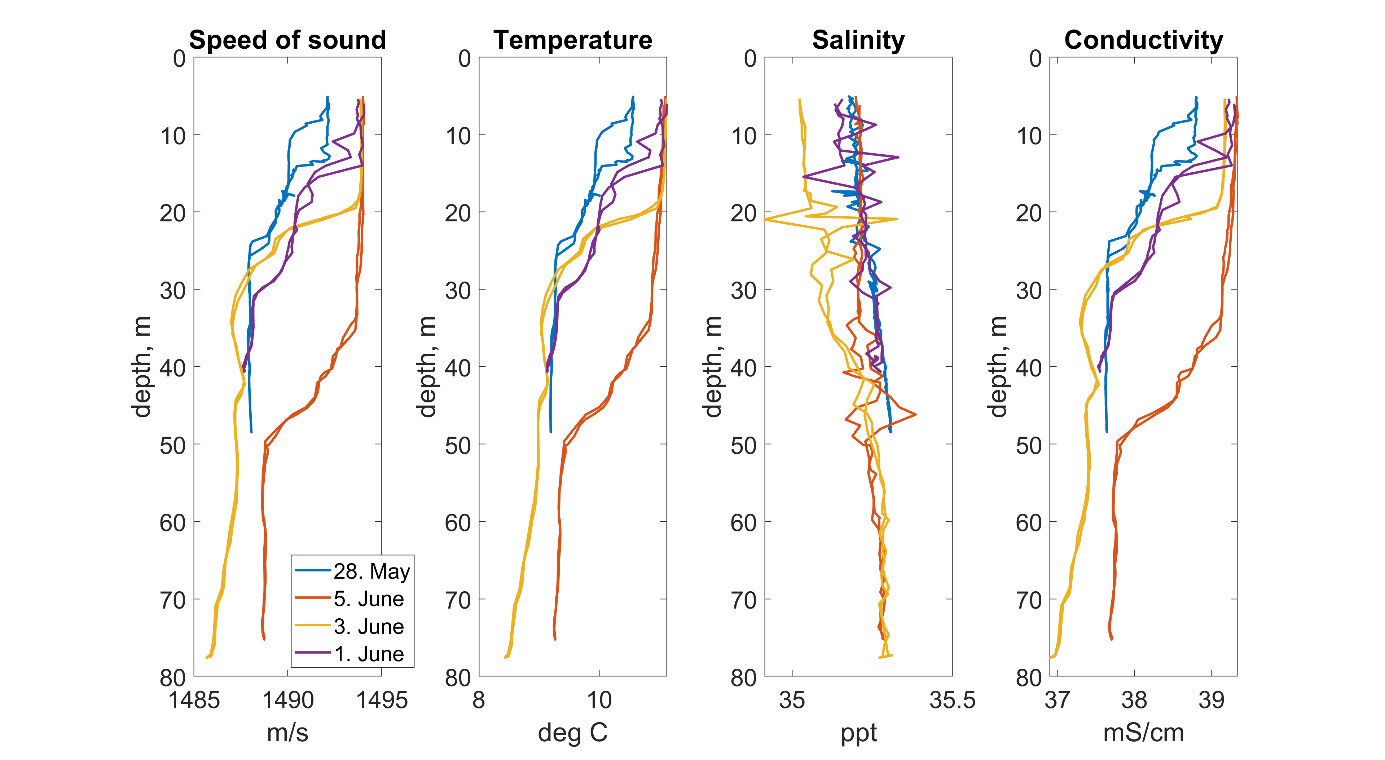
The results from the CTD-measurements are compared in Figure 15 . The echo sounder was updated with averaged CTD-values measured the 28. May ( Table 3 ). CTD-measurements from 1 and 3 June showed only minor variations, so the EK80 settings were not updated. On 5 June, the temperature was slightly higher and therefore the sound speed was also higher, but the EK80 environmental parameters were not updated because the synchronization tool TU40 stopped all synchronized equipment whenever EK80 was stopped. 5 June was a very busy day, with both searching and trawling and no suitable breaks for updating the configuration.
Figure 15 : Comparisons of CTD-measurements during the period of the fisheries.
CTD-saiv
sound speed (m/s)
temperature (°C)
salinity (ppt. )
Conductivity(mS/cm)
28. May
1488.5
9.4
35.2
37.8
01. June
1488.9
9.5
35.3
37.9
03. June
1488.3
9.3
35.2
37.6
05. June
1491.4
10.2
35.2
38.5
Table 3 : Results averaged over depth from 15. meters to the deepest depth.
4.5 - Catch information and Sv(f) of the captured schools
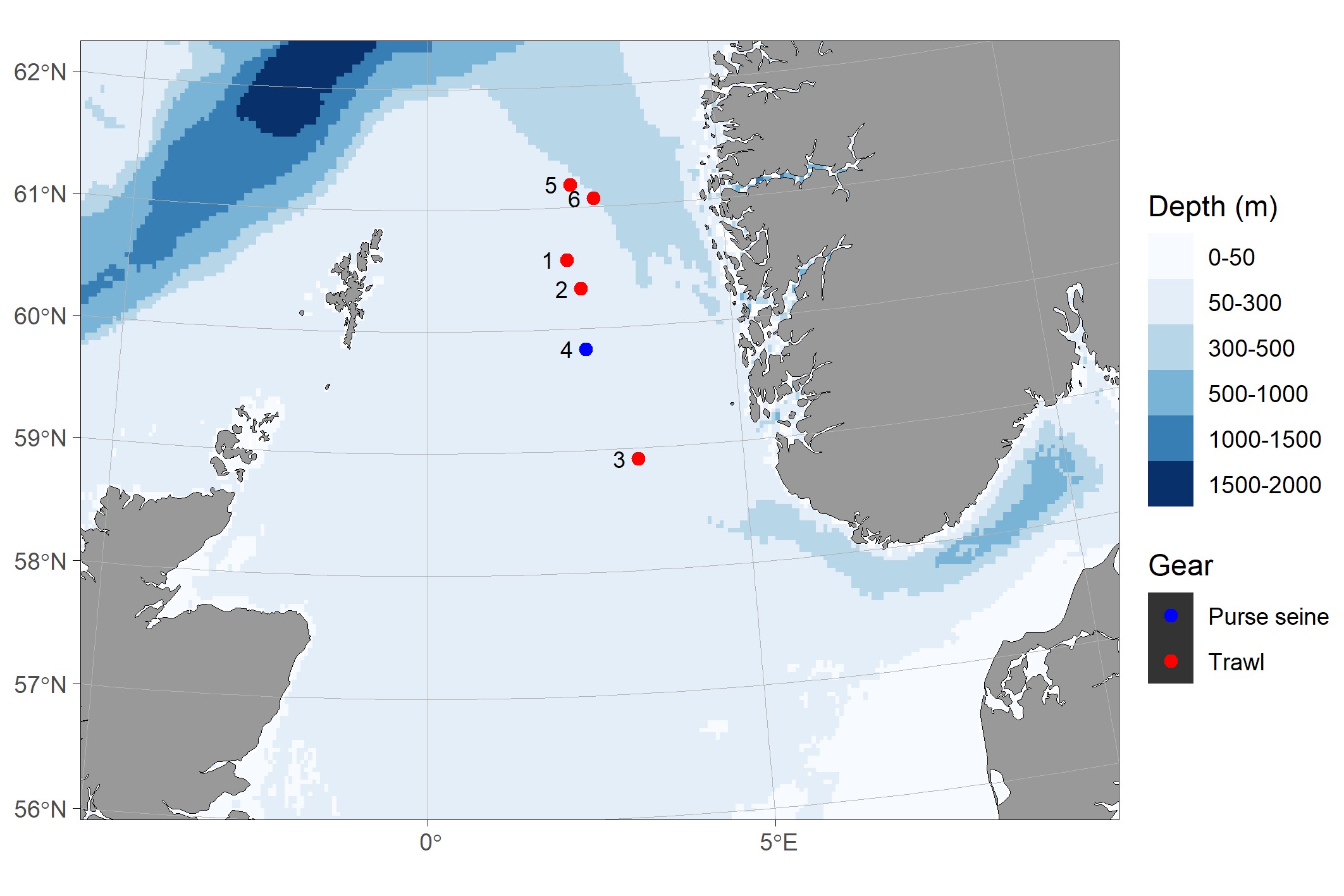
Over the course of the cruise, we made four fishing trips in the Norwegian economic zone in the North Sea close to the border of UK waters (Figure 16). Each trip lasted between one and three days and catches were always landed the day after capture. This resulted in 5 trawl hauls and 4 purse seine sets, but only in one of the purse seine sets th school was caught (Table 3 ).
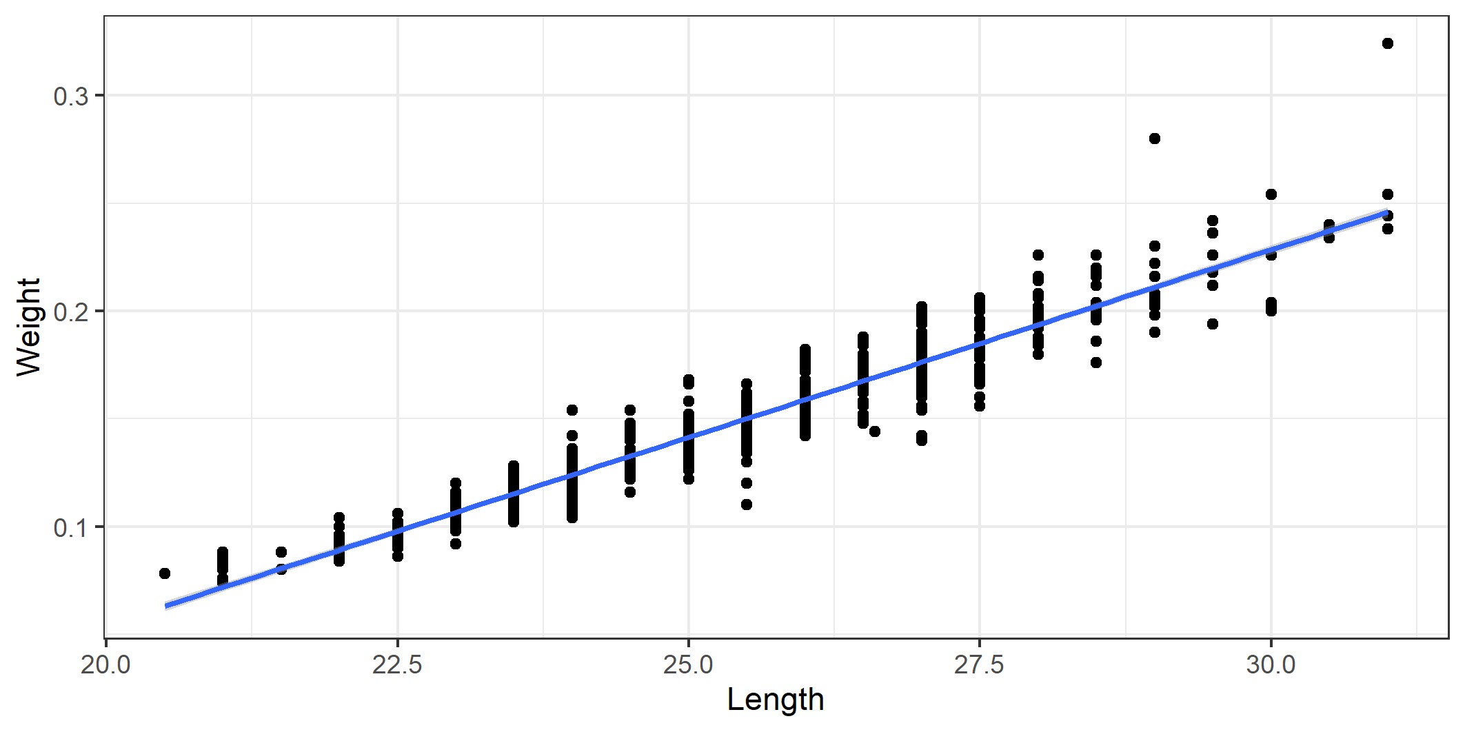
Catch quantities ranged between 40 and 430 tonnes and the by-catch rate of mackerel was between 0 and 0.2 in the catches (Table 3). Average herring length and weight in the catches was between 22.9 and 26.7 cm and 102 and 176 g respective (Figurees 17 and 18). Fishing depths ranged from surface down to seabed, and bottom depth at the fishing grounds was mainly between 90 and 125 m.
Figure 16. Map with catch positions.
Catch
Gear
Start
End
Herring (kg)
Mackerel (kg)
Demersal fish (kg)
1
Trawl
D20260528-T1023
D20260528-T1241
70 000
4 000
500
2
Trawl
D20260528-T1412
D20260528-T1551
70 000
2 000
500
3
Trawl
D20260530-T1345
D20260530-T1717
100 000
874
0
4
Purse seine
D20260601-T1125
NA
40 000
0
0
5
Trawl
D20260605-T0647
D20260605-T0945
418 000
12 000
0
6
Trawl
D20260605-T1205
D20260605-T1429
125 000
25 000
0
Table 4 . Summary of caches during the cruise.
Figure 17 . Herring length and weight distribution in the catches.
Figure 18 . Herring length - weight relationship.
Catch 1 (trawl)
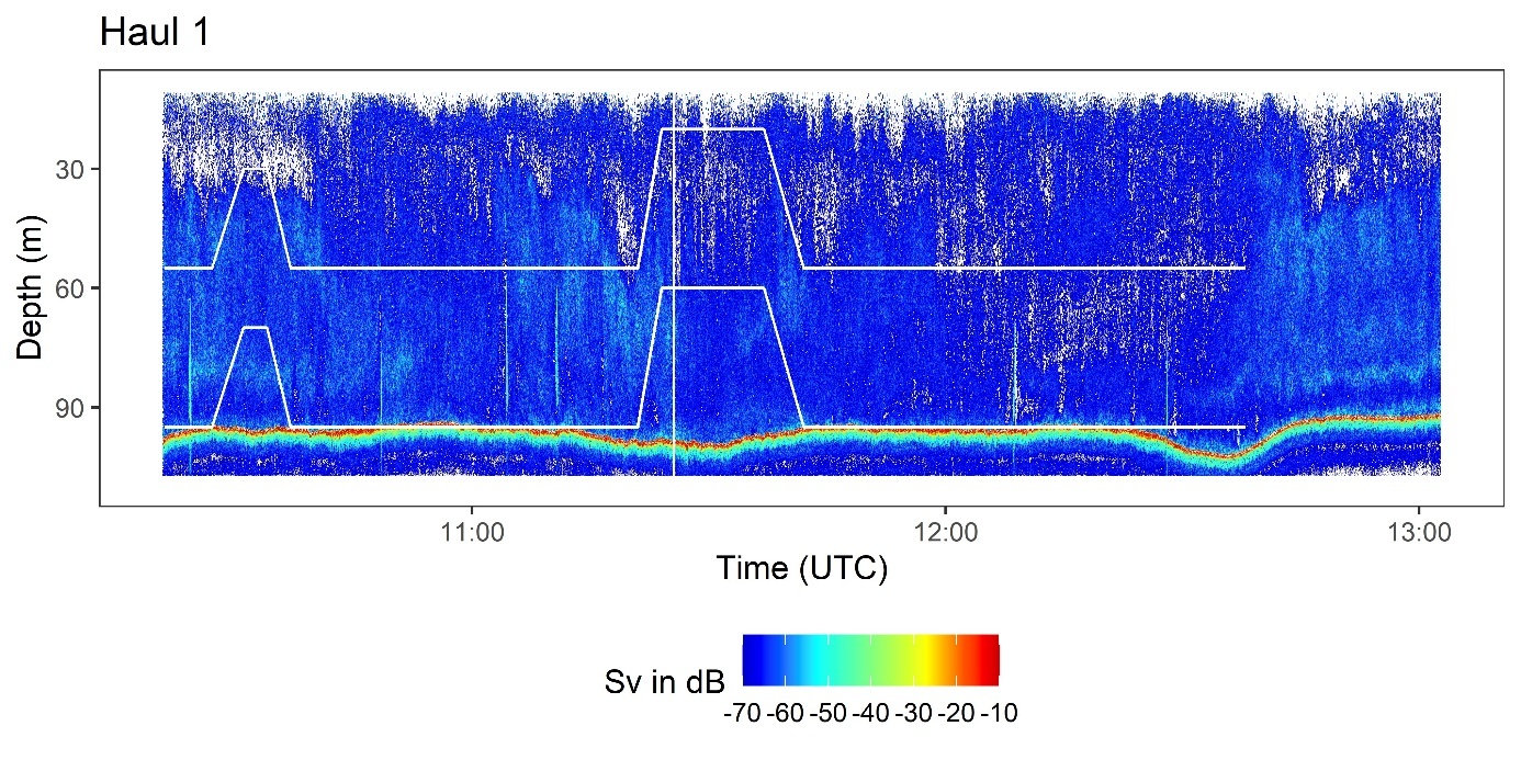
Haul duration was 2 hours and 18 minutes. Six schools, all close to seabed at 60 to 100 m depth, were caught (Figure 19). The catch contained 70 t herring, 4 t mackerel and 500 kg demersal species. Average herring size was 25.2 cm and 0.141 kg. The trawl was mainly on the seabed, but two attempts to catch herring higher up were made. Individual fish were registered near the seabed and small weak schools closer to surface. We did not see any clear indications of where the mackerel were caught.
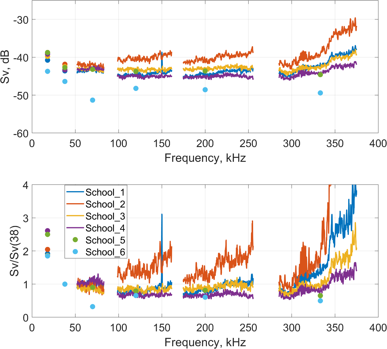
The Sv(f) spectra and the relative Sv(f)/Sv(38 kHz) for each of the six schools (Figure 20) do not display any distinctive features, apart from an apparent increase at 333 kHz. However, this increase is artefactual and results from the limited effective range at 333 kHz due to strong attenuation, which causes elevated noise levels and thus an apparent increase in Sv. Two of the schools were measured with CW settings (marked with dots), while the rest were measured with FM settings.
Figure 19 . Trawl path (white lines) on the echogram - Haul 1.
Figure 20 :Haul 1: Upper plot shows Sv(f) for each herring school in the trawl. Lower panel shows the Sv(f) relative to 38 kHz for the same schools. The apparent increase above 300 kHz is due to noise caused by the limited effective range at high frequencies. School 5 and 6 were measured with narrowband settings.
Catch 2 (Trawl)
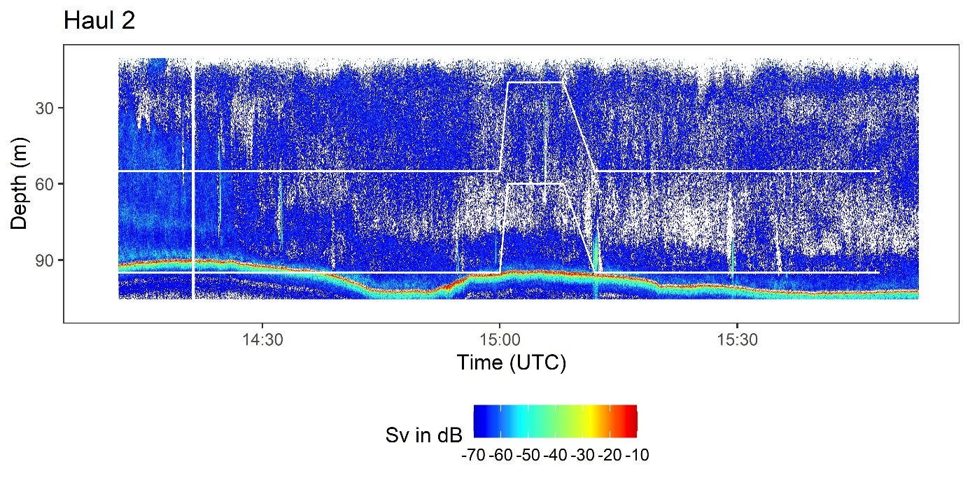
Haul duration was 2 hours and 39 minutes. Seven herring schools, all close to seabed, were caught (Figure 21). The catch contained 70 t herring, 1 t mackerel and 500 kg demersal species. Average herring size was 25.4 cm and 0.144 kg. The trawl was mainly on the seabed. An unsuccessful attempt was made to catch a school higher up in the water column. Individual fish were registered near the seabed and small weak schools closer to surface.
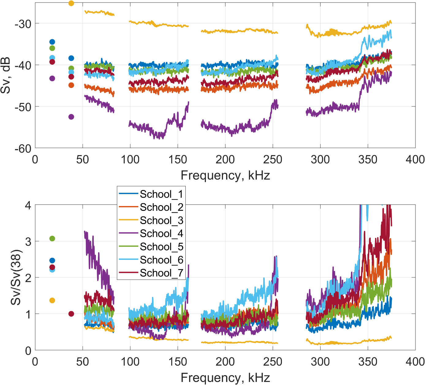
The Sv(f) spectra and the relative Sv(f)/Sv(38 kHz) have a larger variability than for the first catch (Figure 22), two schools show different patterns. Also here the depth causes problems with noise for the 333 kHz transducer resulting in higher Sv values. All the schools were measured with FM settings.
Figure 21 . Trawl path (white lines) on the echogram - Haul 2.
Figure 22 : Haul 2: Upper plot shows Sv(f) for each herring school in the trawl. Lower panel shows the Sv(f) relative to 38 kHz for the same schools. The apparent increase above 300 kHz is due to noise caused by the limited effective range at high frequencies
Catch 3 (Trawl)
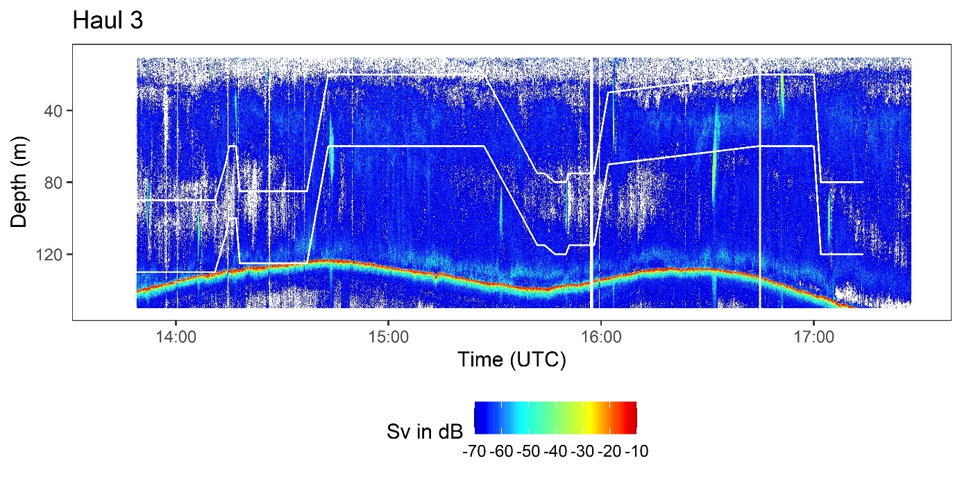
Haul duration was 3 hours and 32 minutes. Seven schools, distributed at varying depths were caught (Figure 23). The catch contained 100 t herring, and 874 kg mackerel. The herring were small, with average size of 22.9 cm and 0.102 kg. Trawl depth varied and was adjusted according to school depths. Individual fish were registered near the seabed and small weak schools closer to surface. The schools in this haul were larger than in the previous hauls.
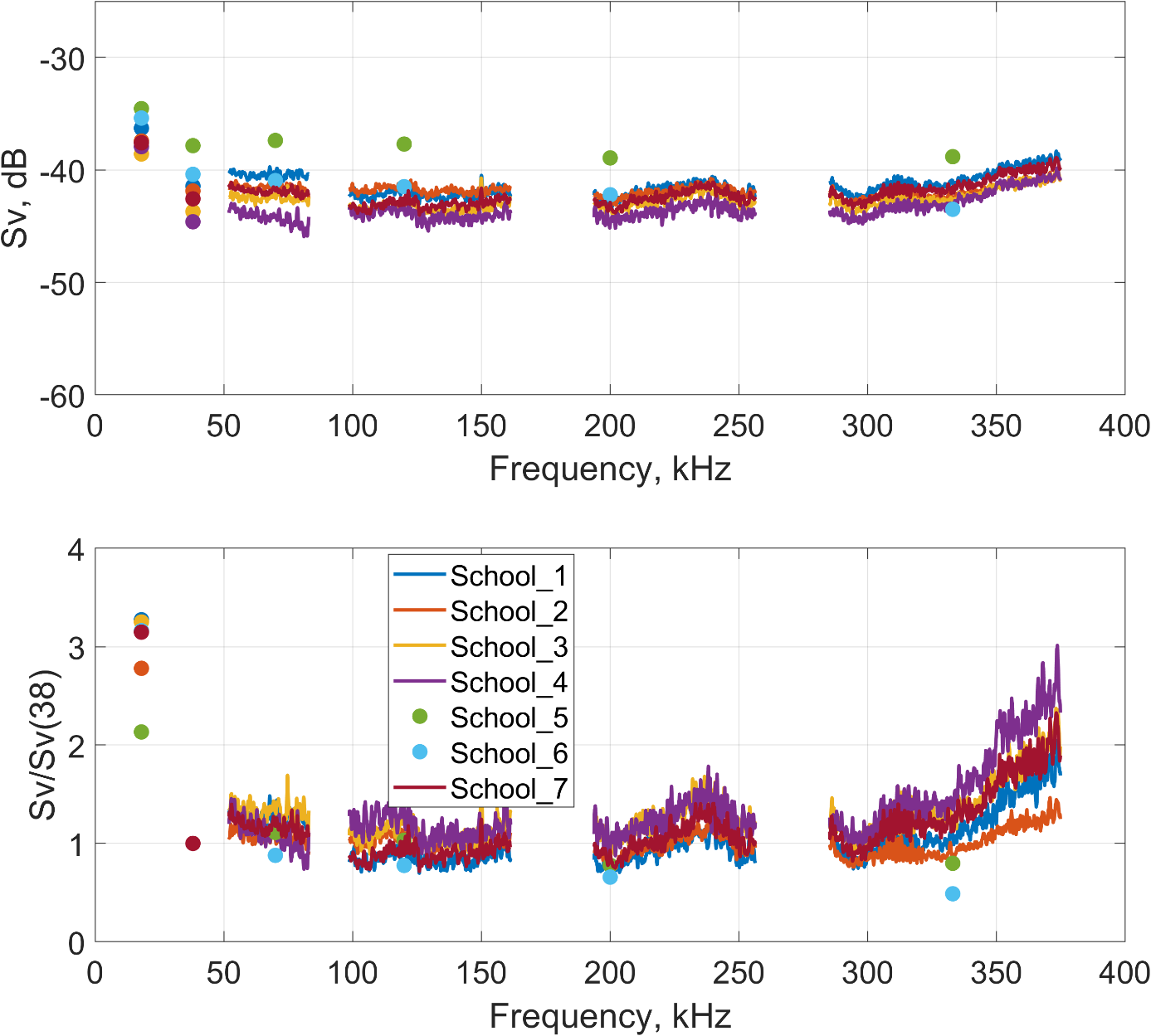
The Sv(f) spectra and the relative Sv(f)/Sv(38 kHz) for the seven schools show much more consistent and closely overlapping patterns (Figure 24), with notably less spread between curves. The size distribution of this catch also showed very little variation, and had the smallest fish observed during our experiments (Figure 17). As in previous cases, the depth introduces noise issues for the 333 kHz transducer, resulting in artificially elevated Sv values. Five schools were measured with FM settings, and two using CW settings.
Figure 23 . Trawl path (white lines) on the echogram - Haul 3.
Figure 24: Haul 3: Upper plot shows Sv(f) for each herring school in the trawl. Lower panel shows the Sv(f) relative to 38 kHz for the same schools The curves are quite consistent, and so was the size distribution for this catch. The depth introduces noise issues for the 333 kHz transducer, resulting in artificially elevated Sv values for this transducer.
Catch 4 (Purse Seine)
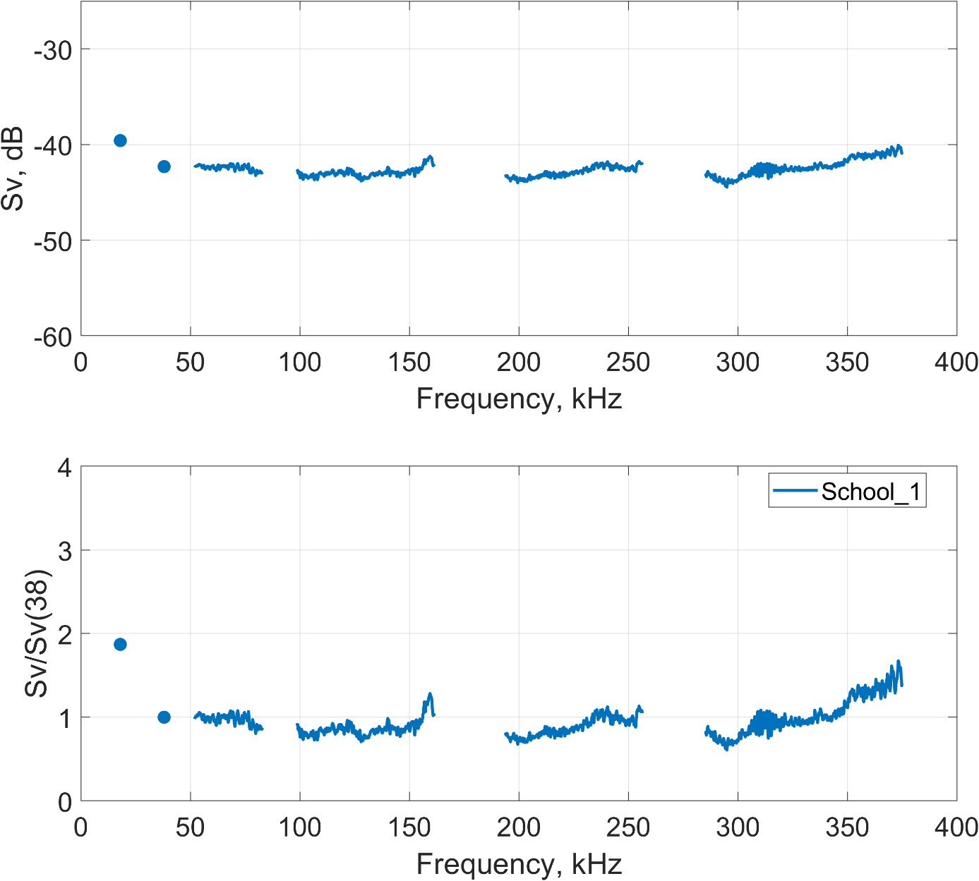
The catch was 40 tonnes of herring with no by-catch of mackerel or other species. The average size of the herring was 25.1 cm and 0.145 kg.
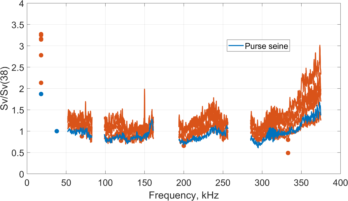
The Sv(f) spectra and the relative Sv(f)/Sv(38 kHz) were plotted for this single school (Figure 25). In this case, trawl-related noise is absent at 18 kHz, providing a more realistic estimate for this frequency than in the previous measurements. The relative Sv(f)/Sv(38 kHz) values are also plotted together with the results from catch 3 (the smallest herring) for comparison ( Figure 26 ). No clear patterns attributable to size differences are apparent.
The Sv(f) spectra and the relative Sv(f)/Sv(38 kHz) were plotted for this single school. In this case, trawl-related noise is absent at 18 kHz, providing a more realistic estimate for this frequency than in the previous measurements. The relative Sv(f)/Sv(38 kHz) values are also plotted together with the results from catch 3 (the smallest herring) for comparison. No clear patterns attributable to size differences are apparent.
Figure 25 : Purse seine no. 1: Upper plot shows Sv(f) for the herring school. Lower panel shows the Sv(f) relative to 38 kHz for the same school.
Figure 26 : Compare sizes: Compare the relative Sv from the schools in trawl haul 3 with average herring length 22.9 cm (orange) and the school from purse seine 1 with 25.1 cm herring length (blue). The 18 kHz form the trawl (orange) is affected by noise.
Catch 5 (Trawl)
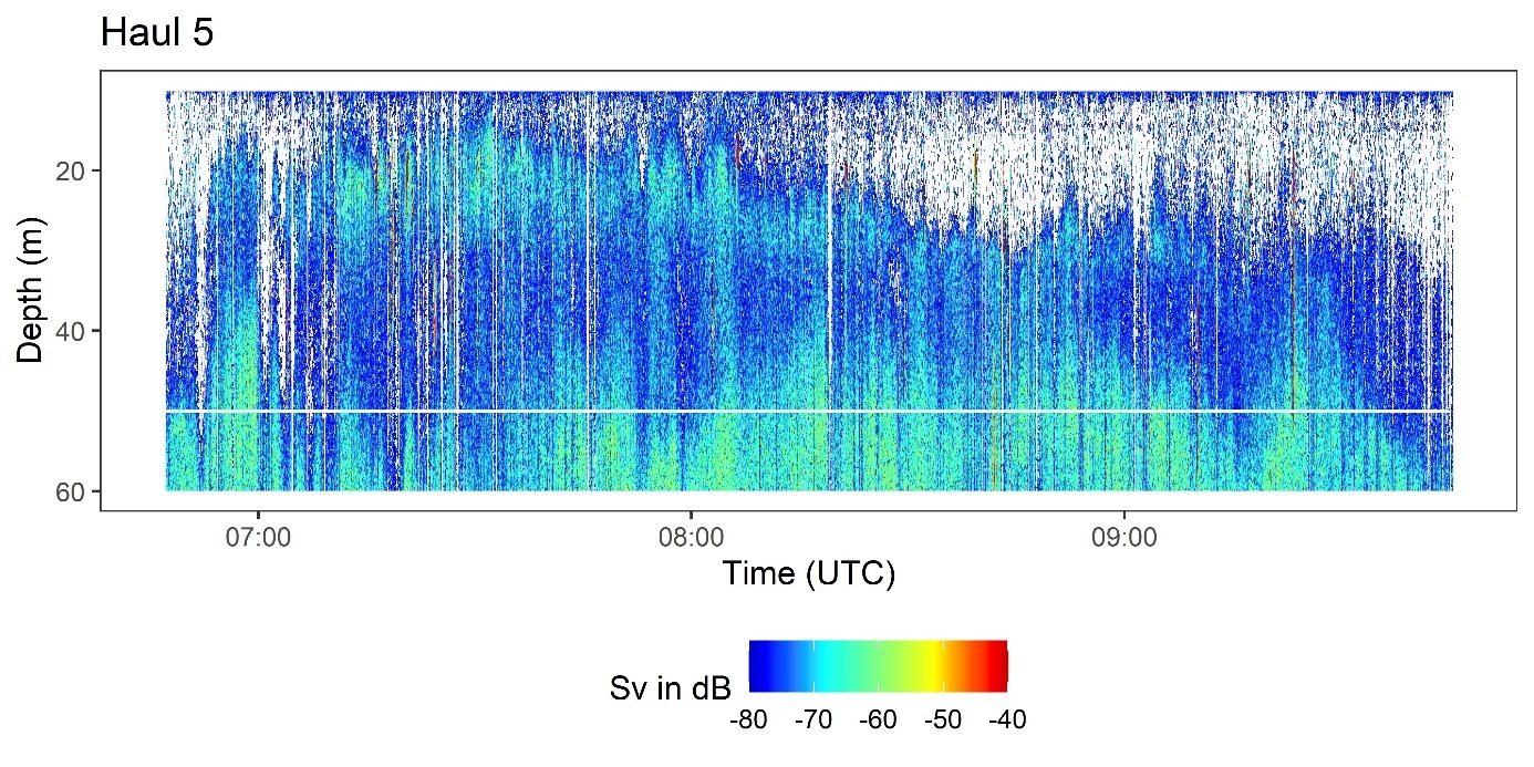
Haul duration was 2 hours and 58 minutes. Several small schools near the surface were caught (Figure 27). The catch contained 418 t herring and 12 t mackerel. Average herring size was 26.7 cm and 0.176 kg. Trawl depth was maintained at same depth, 10 – 50 m.
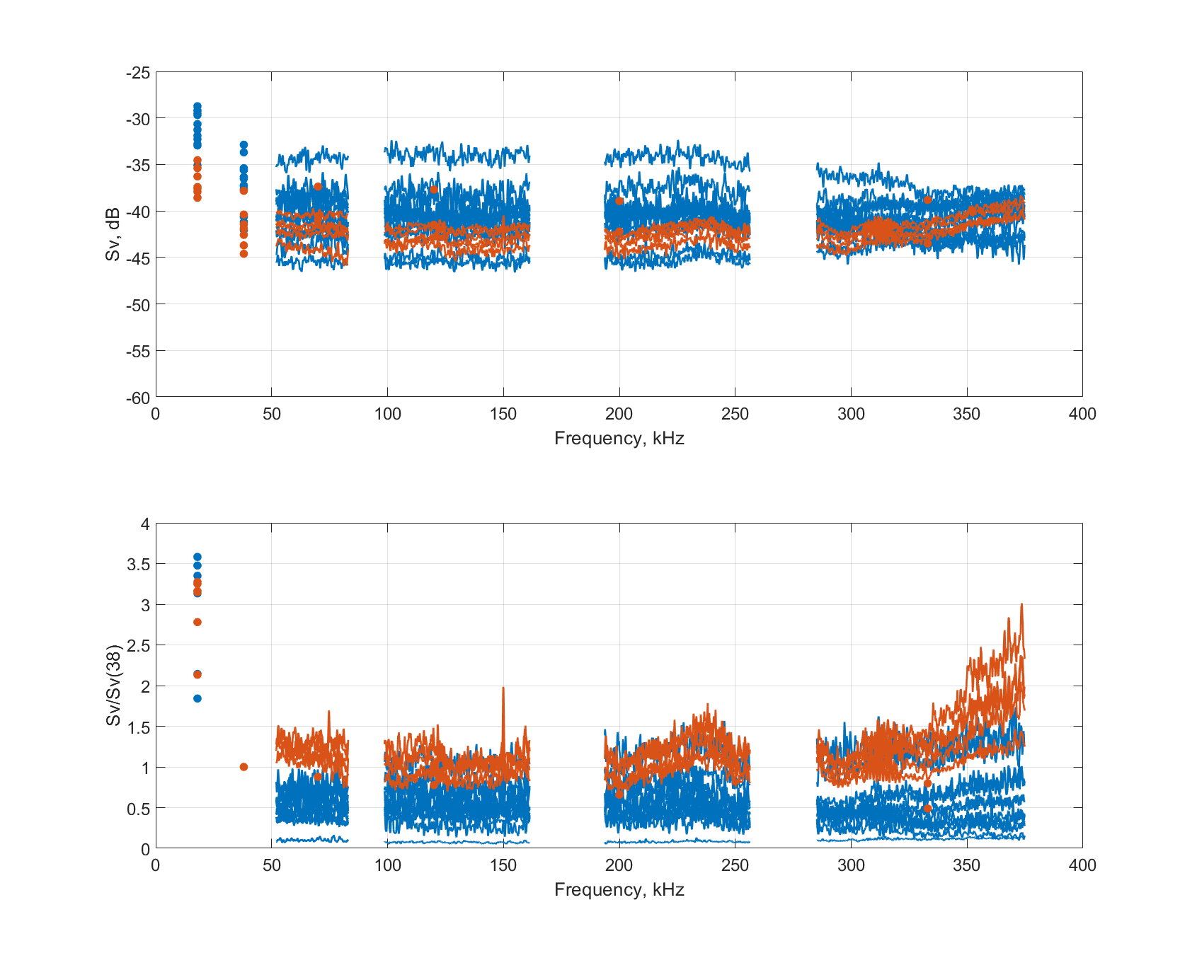
There were 54 schools were many of them were large, while a few were quite small. Plotting the Sv(f) spectra and the relative Sv(f)/Sv(38 kHz) for all schools produced highly chaotic figures, with numerous overlapping curves between -35 and -80 dB. Instead, we selected the largest schools from this day, as the fish caught were relatively large, and compared their the Sv(f) spectra and the relative Sv(f)/Sv(38 kHz) curves with those obtained from the smallest fish in catch no. 3 ( Figure 28 ). Nor here are there any obvious differences attributable to fish size, but the amount of data is too limited to draw firm conclusions. It is conceivable that advanced analysis methods, such as AI-based approaches, could detect subtle patterns not apparent from visual inspection alone.
Analyses using fish identification algorithms in LSSS/Korona was also tested for this catch as described below.
Figure 27 . Trawl path (white lines, 0 – 50 m) on the echogram - Haul 5.
Figure 28 : Compare results between the largest and the smallest fish. Compare Cathc 3 (orange) with Catch 5 (blue). (Different FFT resoultions was used between these results)
Catch 6 (Trawl)
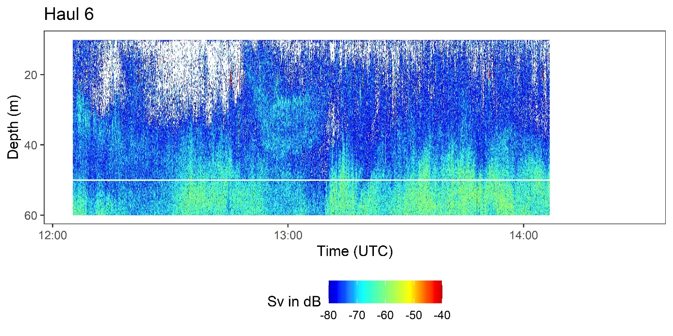
Haul duration was 2 hours and 24 minutes. There was a concern that some of the small aggregations close to surface were mackerel and therefore the trawl was brought in after a relatively short haul (Figure 29) . The total catch was 150 tonnes and contained 25 tonnes mackerel. Average herring size was 27.2 cm and 0.185 kg. Trawl depth was maintained at same depth, 10 – 50 m. depths.
The echosounder data revealed around 90 schools in the 10–50 m layer, most of which were very small. The frequency responses of these schools were plotted and compared, but they did not provide any additional insight beyond what was already demonstrated in the previous trawl examples. For this catch, the analysis therefore focused primarily on fish identification algorithms in Korona/LSSS.
Figure 29 . Trawl path (white line indicates the bottom of the trawl) on the echogram - Haul 6.
4.6 - Detection of mackereland herring
Q: Does the mackerel-detection algorithm incorporated in KORONA work well in noisy data?
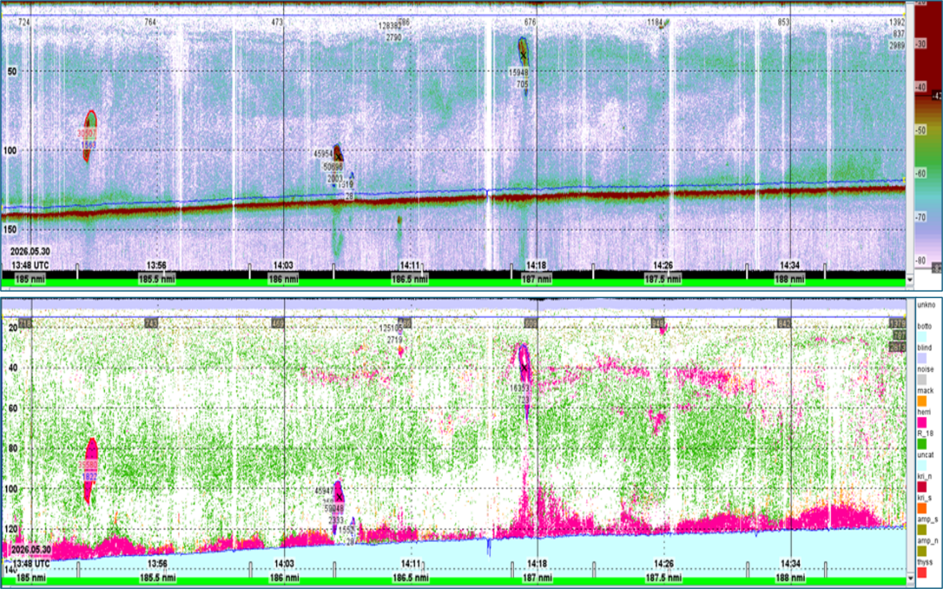
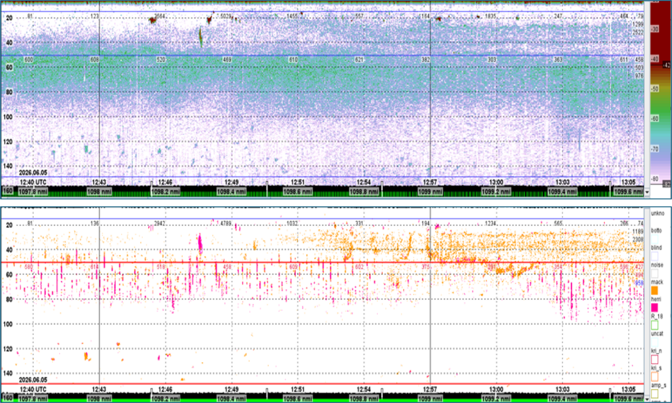
Figure 30 show result of KORONA algorithm for detection of acoustic categories (“species”) herring, no mackerel. The green background-layer shows targets with a small gas-inclusion. The catch of Trawl station 3 showed 99% herring of the 100 metric ton catch.
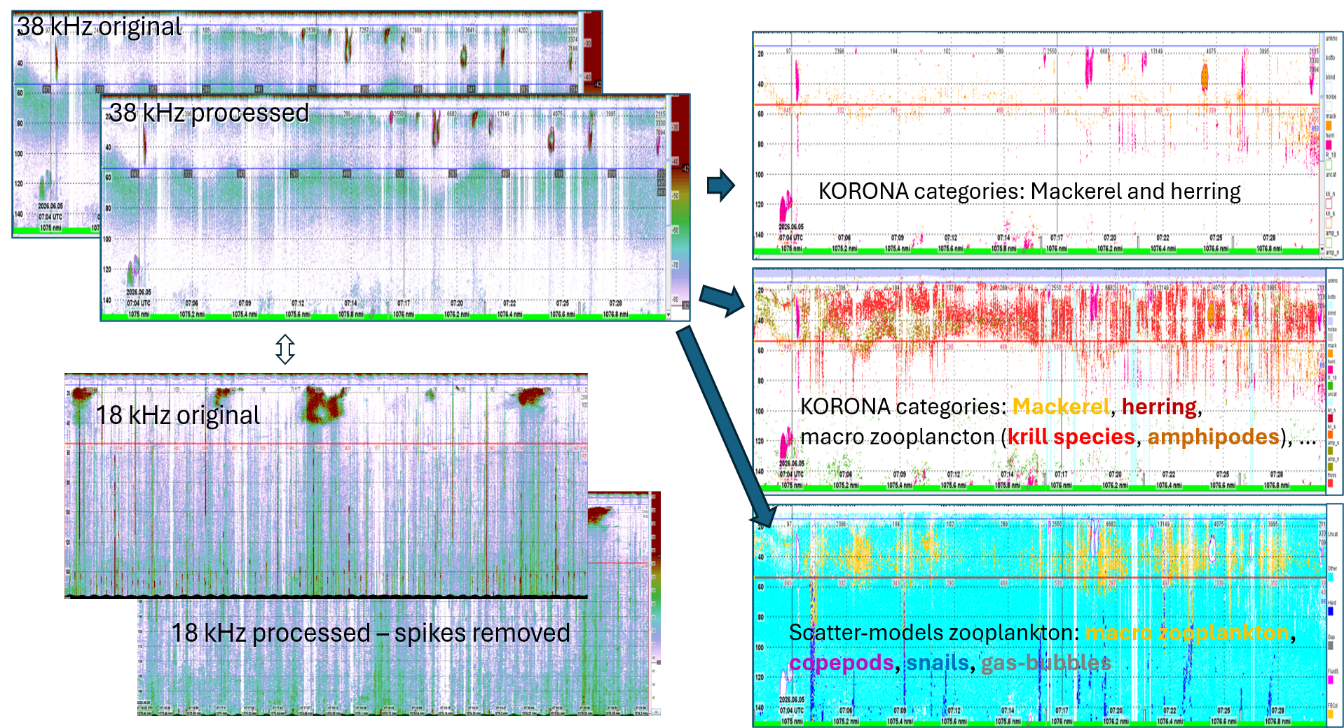
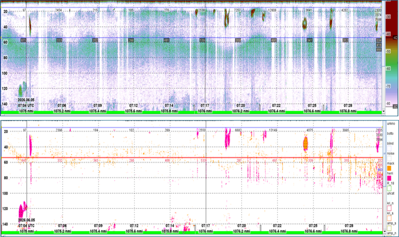
Figure 31 shows that both herring and mackerel were apparent in Trawl station 5 (418 t catch, 97% herring), with large amounts of krill in the background layer. Figure 32 zoom up by showing only the original 38 kHz data and the pixels where KORONA has detected either mackerel or herring. Krill is invisible (white). Figure 33 shows detections of mackerel (orange) and herring (purple) from trawl station 6 with krill invisible as they are shown in white colour. There were 80% herring in the 125 metric ton catch.
Trawl stations 5 and especially 6 was reported as especially challenging as there were mixtures of herring and mackerel.
Figure 30 . Echograms during trawl station 3 (herring only). Automatic identification gave herring and no mackerel. The green background shows targets resonant at 18 kHz (gas-inclusion of 1 m diameter) which indicates very small fish with swimbladder or jellyfish with a gas inclusion.
Figure 31. In trawl station 5 KORONA found herring and mackerel with krill in the background. Data contained much spike-noise at 18 kH (lower left).
Figure 32. Trawlstation 5. 38 kHz echogram and KORONA detections of herring (pink) and mackerel (orange). Krill i bakgrunnen vises ikke (hvit farge).
Figure 33. Trawl station 6. 38 kHz echogram and KORONA detections of herring (pink) and mackerel (orange). Krill detections have been removed(white colour).
4.7 - Advantages and disadvantages using acoustic broadband compared to narrowband
The higher along beam resolution in FM is expected to make detection of individual mackerel and small aggregations in 200 kHz easier. Acoustic broadband could also make species identification better than acoustic narrowband, but the current LSSS acoustic feature-library has not incorporated acoustic broadband (yet), although this is just a job that could be done even with the current version of LSSS.
EK80 can use either acoustic broadband (FM) or acoustic narrowband (CW). The advantages using broadband is better spatial and frequency resolution in pelagic data. One disadvantage is the increased amount of data. Another disadvantage is the poorer bottom detection when using FM due to the need for using a FFT-window (this is a technical detail). There could be more noise in broadband data, at the same time as improved processing techniques could reduce noise. An advantage is that broadband data can be split into several sub-channels with the purpose of improved species identification. If the frequencies of the sub-channels are standardized, the acoustic feature-library could be expanded. Unfortunately, the existing feature-library that was used on the Eros-survey was not expanded, which in turn did not result in improved species identification.
Furthermore, the use of acoustic broadband does not necessarily mean the use of linear up-sweep CHIRP (or even CHIRP in general). It is possible to use broadband to transmit very short pulses in the current EK80. In general, it should be possible to transmit several pulses with different centre frequencies simultaneous from one transducer. That would, however, require a modification of the EK80 software that controls the WBT. Furthermore, the transducer should have frequency-independent beamwidth for the acoustic data at different frequency to be comparable.
5 - Conclusions and recommendations
By-catch of mackerel is a problem in the NS herring fishery and there is a need to develop practical methods for improved detection of mackerel. Mackerel and herring co-occur in the same area in small loose aggregations or larger schools (herring). The impression is that herring and mackerel do not occur in mixed schools and the purse seine catches seldom contain mackerel, but there is no definitive evidence for it.
During trawling the schools are first seen on the sonars, then on the keel mounted EK80 echosounders. When the school is observed on the echosounder there is still time to adjust the position of the trawl to either try to catch or to avoid the school. Reliable methods to detect and identify mackerel with the echosunders in real time would be highly useful for the fishermen.
Mackerel and herring have different acoustic properties, but the challenge is that mackerel is a weak target and occur in loose aggregated making it difficult to detect. The preliminary results indicate that it was possible to detect small aggregations of mackerel close to surface. These detections seem to match with the trawl catches. The results from the automatic species detection in korona also support this. However, it remains to be determined whether the detection is sufficiently accurate. More work is also needed to dteremine what frequency bands are required.
Another challenge in the fishery is undersized herring. Due to the dense schools it was not possible to measure the target strength (TS) of individual herring, this will probably be generally difficult to measure in situ. Methods for sizing of herring with broadband echosounders would probably have to focus on the Sv(f). We focused mainly on species identification in this survey, but we had one haul with clearly (~2.5 cm averag difference) smaller herring. We compared the Sv(f) between schools of large herring and small herring, but there was no clear difference in the Sv(f) between the different size groups. We cannot rule out the possibility that Sv(f) can be used to distinguish between herring of different sizes. However, we have too little data in this study. If we had a large dataset of Sv(f) from herring of known size, we could try to train AI-based algorithms to recognize size classes. Such a dataset is currently not available, so this remains an open question for future research.
5.1 - Synchronization & Noise
TU40 is a useful tool for synchronization. All instruments that are possible to synchronize should be synchronized. A delay of 2 times the depth divided by the speed of sound should be applied as a starting point for a given pulse repetition rate. Instrument settings (e.g. frequency bands, pulse lengths and operational ranges and tilt angles) and environmental conditions (e.g. bottom depth) affect synchronization. Therefore, during operation the delay needs to be adjusted when noise is detected on the EK80 display.
ST90 was most difficult to adjust since it has vertical beams and a horizontal fan with long ranges. The captain wanted a low frequency on the horizontal fan, 14 kHz, which conflicts with the 18 kHz transducer in CW. The vertical beam range was shorter and did therefore not require such a low frequency. The vertical beams were set to 22 kHz which removed the noise on EK80. The noise from the long pulses of the fan is still difficult to remove completely. In our case it helped to increase the ping interval of EK80 to 500 ms to make more “space” for the noise.
For instruments that cannot be synchronized such as the Furuno Sonar FSV75 an alternative to consider for broadband is to reduce the bandwidth to avoid the interfering frequencies. In this case FSV75 uses 180 kHz which was avoided by changing the start of the 200 kHz band from 170 to 190 kHz.
5.2 - Broadband vs narrowband
Higher range resolution of broadband makes it easier to detect weak single individuals and small aggregations of mackerel. Using (only) the the 200 kHz transducer with broadband settings may therefore improve detection. Broadband could possibly also improve species identification, but the current LSSS acoustic feature library has not incorporated broadband and it was not possible to test on these data yet. On the other hand, broadband echosounders are expensive, generate large amounts of data and introduce more noise and should not be used unless it is necessary. It remains to investigate whether weak mackerel targets can be detected without having the 200 kHz transducer in broadband mode. As mentioned above broadband may potentially also be useful for size determination of herring.
5.3 - Suggestions for how to move forward
Evaluate the results from the species identification models in ES80 and LSSS /Korona. How well do they match the species distribution in the catches and is the performance good enough?
Investigate whether species detection improves when different degrees of broadband is used.
Establish good routines for synchronization and noise reduction for the settings that are needed for the species identification. As part of this work, an evaluation of whether trawl door noise can be removed from the 18 kHz echosounder may be required.
Evaluate how avoidance behaviour may affect the frequency response.
Some sonar and echosounder software (ES80, SEAPIX, Furuno) have already tools for species identification. These are generally based on different relative responses on two frequencies. In the ES80 software it is also possible to teach the system what acoustic responses corresponds with what species. Based on discussions on EROS our impression is that even though this function is available it is not in use. We need a better understanding of to what degree the existing methods are used during commercial fishing and what the reasons for not using them are where this is the case.
6 - Acknowledgements
We would like to thank Pål Cato Reite and the crew on Eros and Kongsberg Discovery for good cooperation and support during the planning and conducting the experiment.
7 - References
Demer, D.A., Berger, L., Bernasconi, M., Bethke, E., Boswell, K., Chu, D., Domokos, R., Dunford, A., Fassler, S., Gauthier, S., Hufnagle, L.T., Jech, J.M., Bouffant, N., Lebourges-Dhaussy, A., Lurton, X., Macaulay, G.J., Perrot, Y., Ryan, T., Parker-Stetter, S., Stienessen, S., Weber, T., Williamson, N., 2015. Calibration of acoustic instruments. (Report). International Council for the Exploration of the Sea (ICES). https://doi.org/10.25607/OBP-185
Korneliussen, R. (Ed.), 2018. Acoustic target classification. ICES Cooperative Research Report No. 344, 104pp.
Korneliussen, R.J., Heggelund, Y., Eliassen, I.K., Johansen, G.O., 2009. Acoustic species identification of schooling fish. ICES J Mar Sci 66, 1111–1118. https://doi.org/10.1093/icesjms/fsp119
Korneliussen, R.J., Heggelund, Y., Macaulay, G.J., Patel, D., Johnsen, E., Eliassen, I.K., 2016. Acoustic identification of marine species using a feature library. Methods in Oceanography 17, 187–205. https://doi.org/10.1016/j.mio.2016.09.002
Kubilius, R., Bergès, B., Macaulay, G.J., 2023. Remote acoustic sizing of tethered fish using broadband acoustics. Fisheries Research 260, 106585. https://doi.org/10.1016/j.fishres.2022.106585
Nøttestad, L., Diaz, J., Penã, H., Søiland, H., Huse, G., Fernö, A., 2016. Feeding strategy of mackerel in the Norwegian Sea relative to currents, temperature, and prey. ICES Journal of Marine Science 73, 1127–1137. https://doi.org/10.1093/ICESJMS/FSV239