This is the survey report for IMR survey number 2022812 in the project “SpawnSeis MV”. The purpose of the survey was to expose spawning cod to sound a marine vibrator; a continuous transmitting seismic source. The exposure was conducted from FFI`s research vessel “H.U. Sverdrup II” and the sound exposure by the vibrator “BASS”, developed by Shearwater Geoservices. The survey was carried out in the period February 12-18 th 2022. in an area in Austevoll south of Bergen were a telemetry network to track cod is established. Additionally, sound measurements were conducted during the entire week, and results of these are presented in this report.
SpawnSeis MV exposure experiment - Survey Report
— IMR Survey number 2022812
Report series:
Toktrapport 2023-4
ISSN: 1503-6294
Published: 14.03.2023
Updated: 12.04.2023
Cruise no.: 2022812
Project No.: 15819
On request by: Havforskningsinstituttet, Equinor Energy AS, Lundin Energy Norway AS, ENI Vår Energy AS, Reflection Marine Norge AS
Research group(s):
Økosystemakustikk
Subject:
Seismikk,
Biologisk lyd
Program:
Nordsjøen
Research group leader(s):
Rolf Korneliussen (Økosystemakustikk)
Approved by:
Research Director(s):
Geir Huse
Program leader(s):
Henning Wehde
Norsk sammendrag
Summary
Dette er toktrapport for toktnummer 2022812 i prosjektet «SpawnSeis MV». Hensikt med toktet var å eksponere gytende torsk for lyd fra en marin vibrator som er en kontinuerlig seismikk-kilde. Eksponeringen ble utført med FFI sitt forskningsfartøy «H.U. Sverdrup II» og lydeksponeringen med vibratorkilden «BASS», utviklet av Shearwater GeoServices. Toktet ble utført i perioden 12-18.februar 2022 i et område på Austevoll hvor det er etablert et telemetri-nettverk for å spore merket torsk. Det ble også utført lydmålinger under hele uken, og resultatene fra disse er presentert i denne rapporten.
1 - Introduction
In the project SpawnSeis MV, we aimed to study how a novel seismic source, a marine vibrator, affects behaviour and acoustic communication of wild, free ranging, spawning cod. Cod behaviour was studied by using acoustic telemetry to track movement of individual cod in Austevoll, Norway (Fig. 1). During the cod spawning season in 2020 and 2021, a 5-day exposure survey with seismic airguns was used to examine cod movement in response to such sound exposure. In the spawning season of 2022, an exposure survey with a marine vibrator was conducted to evaluate differences between how cod respond to these two types of seismic testing (airguns and marine vibrator). The current cruise report describes the exposure survey with the marine vibrator. The airgun surveys are described in Sivle et al. (2021).
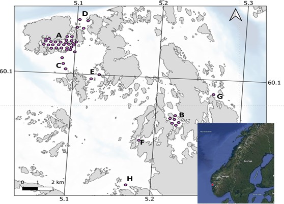
Figure 1. A total of 36 acoustic telemetry receivers in two grids in the Austevoll archipelago; in Bakkasund spawning area (A), a smaller grid in Osen spawning area (B), as curtains to control the western (C), northern (D) and southern (E) gateway from the main area as well as 3 additional spawning sites in the area (F, G, H). A total of 80, 77 and 50 cod were tagged in the years 2020;21 and 22, respectively. Additional details can be found in McQueen et al. (2022).
The current survey, conducted in February 2022 was a 5-day exposure with a marine vibrator, the Broadband Acoustic Seismic Source (BASS), in Bakkasund (Fig. 1). February was chosen to coincide with the main spawning period of the cod, and the previous two surveys with airguns were conducted within the same time-period to allow for comparisons between years.
Whereas conventional seismic sources (airguns) transmit a short broadband impulse signal with a high peak pressure, marine vibrators transmit continuous frequency modulated sweeps within a much narrower band, at lower peak pressure levels, but not necessarily with lower total energy levels. The purpose of this survey was to compare the behavioural responses of cod at a spawning site when exposed to a seismic source transmitting continuously to the behavioural responses of the cod when exposed to the more conventional pulsed signal from the airgun used in 2020 and 2021. The sound exposure level (SEL) was intended to be as similar as possible for the two types of sources, although the waveform and the frequency spectra were very different. In the previous 2 years with the seismic airguns, the source was towed behind the vessel along a “racetrack” (Sivle et al. 2021). The version of BASS used in the current experiment cannot be towed and was therefore instead lowered from the anchored vessel. The sound level of the stationary source was varied to mimic the variation caused by a moving vessel with increasing and decreasing distances between the source and the spawning ground
This survey report contains a description of the methods and the experiment conducted and some dataplots of the measurements taken during the survey, but no analyses of these data.
2 - Methods
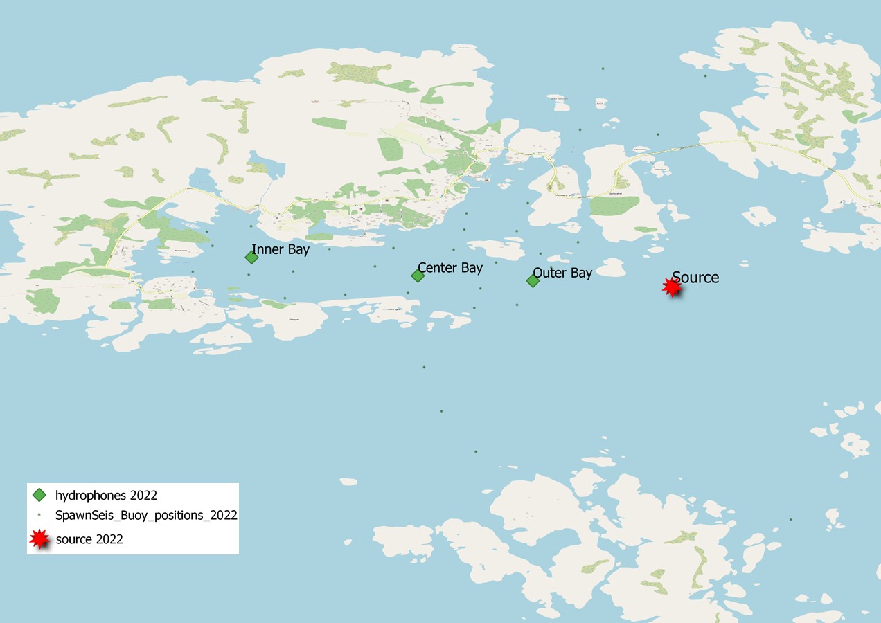
The exposure experiment was conducted by having the marine vibrator deployed stationary from a ship placed just outside the main telemetry grid in Bakkasund (Fig 2). More details of the telemetry grid and fish tagging can be found in McQueen et al. (2022). The sound from the marine vibrator, as well as the background sound between exposures, were recorded at three different hydrophones placed at various distances from the source (Fig 2; inner, center and outer bay), thus measuring the received sound levels at various positions inside the cod spawning location.
2.1 - Vessel
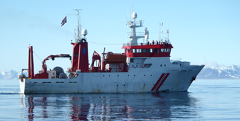
The survey was conducted between February 12th and February 18th 2022 with the Norwegian Defence Research Establishment (FFI)`s research vessel “H.U. Sverdrup II” (Fig 3). This was the same vessel that was used for the airgun exposures conducted in 2020 and 2021.
2.2 - Scientific crew
Personnel from Norwegian Defence Research establishment (FFI), Institute of Marine research (IMR) and Shearwater GeoServices (SGS) participated in the survey. A list of the personnel and their tasks are given in Table 1.
| Name | Institution | Main role |
| Petter Kvadsheim | FFI | Cruise leader FFI cruise coordinator Coordinate ongoing operation |
| Kari Wegger Ektvedt | FFI | Operate hull mounted hydrophones/ help ongoing operation |
| Lise Doksæter Sivle | IMR | HI Cruise coordinator /help ongoing operations |
| Kate McQueen | IMR | Help ongoing operations |
| Erik Schuster | IMR | Operate hydrophones in exposure area |
| Sigurd Hanaas | IMR | Operate hydrophones in exposure area |
| Lars-Oskar Westavik Gaustad | SGS | Operate MV source |
| Richard Graham Forrester | SGS | Operate MV source |
| Mark Ozimek | SGS | Operate MV source |
| Benjamin Whiting | SGS | Operate MV source |
| Ricardo Quintanilla | SGS | Operate MV source |
2.3 - Marine Vibrator BASS
The marine vibrator (MV) used in this survey is called BASS (Fig 4) and is developed by Shearwater GeoServices. In contrast to the exposure with airguns in the previous years, BASS will be used as a stationary source, as the prototype MV is not yet built into a tow body.
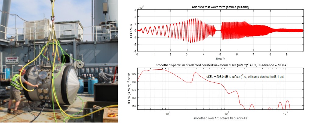
BASS has a nominal bandwidth of 3-150 Hz. BASS is designed to be able to emit sound continuously without any gap or listening period. In commercial applications, several vibrator units will be used together, each operating in a dedicated segment of the nominal band. The vibrators emit sound continuously, although it can be used with silent gaps if required.
For SpawnSeis MV experiment only one vibrator was used, operating over the full nominal bandwidth. The sweep used was a concatenation of two individual sweeps that would normally be emitted simultaneously from two vibrators (Fig 4).
2.4 - Exposure design
We aimed at mimicking the exposure design of the airgun exposure as used in 2020 and 2021, with 9 hours blocks consisting of three exposure conditions (Sivle et al. 2021). These conditions included active sound transmission and 2 types of control (silent control: no transmission, vessel left the area, boat control: no transmission, vessel on the exposure track), each block lasting 3 hours. Therefore, in the current survey, we aimed to expose the cod for three hours of transmission in each 9-hour block. The reasoning for the previous year`s boat control was to exclude potential reactions to the vessel noise from the seismic noise. This year, however, with the stationary vessel without running engines no such control was needed. During the entire experiment, the main engine was turned off. The shipd`s main generator was running to provide electricity to the ship, and the BASS source was powered by an own generator. The control in the current survey was therefore that the vessel simply stayed onsite at anchor with the source in the water and all engines turned off, except the main generator.
The three exposure types used were thus:
-
3 hrs of active transmission with the BASS source (BASS)
-
3 hrs of silent, only main generator running (silent 1)
-
3 hrs of silent, only main generator running (silent 2)
The order of the sessions was fully randomized within blocks (Table 2). Silent 1 and silent 2 sessions are equal.
| Block Number | Treatment | Start | End |
| 1.1 | BASS | T0 | T0+3hrs |
| 1.2 | Silent control 1 | T0+3 | T0+6 |
| 1.3 | Silent control 2 | T0+6 | T0+9 |
| 2.1 | Silent control 2 | T0+9 | T0+12 |
| 2.2 | BASS | T0+12 | T0+15 |
| 2.3 | Silent control 1 | T0+15 | T0+18 |
| 3.1 | Silent control 2 | T0+18 | T0+21 |
| 3.2 | Silent control 1 | T0+21 | T0+24 |
| 3.3 | BASS | T0+24 | T0+27 |
| 4.1 | Silent control 2 | T0+27 | T0+30 |
| 4.2 | BASS | T0+30 | T0+33 |
| 4.3 | Silent control 1 | T0+33 | T0+36 |
| 5.1 | BASS | T0+36 | T0+39 |
| 5.2 | Silent control 1 | T0+39 | T0+42 |
| 5.3 | Silent control 2 | T0+42 | T0+45 |
| 6.1 | Silent control 2 | T0+45 | T0+48 |
| 6.2 | BASS | T0+48 | T0+51 |
| 6.3 | Silent control 1 | T0+51 | T0+54 |
| 7.1 | Silent control 1 | T0+54 | T0+57 |
| 7.2 | Silent control 2 | T0+57 | T0+60 |
| 7.3 | BASS | T0+60 | T0+63 |
| 8.1 | BASS | T0+63 | T0+66 |
| 8.2 | Silent control 2 | T0+66 | T0+69 |
| 8.3 | Silent control 1 | T0+69 | T0+72 |
| 9.1 | Silent control 1 | T0+72 | T0+75 |
| 9.2 | BASS | T0+75 | T0+78 |
| 9.3 | Silent control 2 | T0+78 | T0+81 |
| 10.1 | Silent control 2 | T0+81 | T0+84 |
| 10.2 | Silent control 1 | T0+84 | T0+87 |
| 10.3 | BASS | T0+87 | T0+90 |
The aim was to conduct 10 exposure sessions in total, to expose the fish to the same total dose as for the airguns. Therefore, plan A was to conduct a full set with 2 control sessions (silent 1 and silent 2) per block, but if time became short, silent 2 would be excluded to enable reaching the aim of 10 exposure sessions.
The first block started on the evening of day 2, February 13th, 2022. Hence it was considered sufficient time to finalize all 10 blocks with 3 sessions each (BASS-silent1-silent2). However, on the morning of day 5 (February 16th ) an incident with the source with massive water intrusion caused a 12 hr delay in the experimental program. Therefore, it was decided to skip one control session in each remaining block, to be able to conduct 10 exposure sessions. Silent 2 was therefore skipped in the remaining blocks; 8, 9 and 10. The final treatment schedule is shown in Table 3.
| Block/Session | Treatment | Start (UTC) | End (UTC) |
| 1.1 | BASS | 13.02.2022 19:35 | 13.02.2022 22:35 |
| 1.2 | Silent control 1 | 13.02.2022 22:35 | 14.02.2022 01:35 |
| 1.3 | Silent control 2 | 14.02.2022 01:35 | 14.02.2022 04:35 |
| 2.1 | Silent control 2 | 14.02.2022 04:35 | 14.02.2022 07:35 |
| 2.2 | BASS | 14.02.2022 07:35 | 14.02.2022 10:35 |
| 2.3 | Silent control 1 | 14.02.2022 10:35 | 14.02.2022 13:35 |
| 3.1 | Silent control 2 | 14.02.2022 13:35 | 14.02.2022 16:35 |
| 3.2 | Silent control 1 | 14.02.2022 16:35 | 14.02.2022 19:35 |
| 3.3 | BASS | 14.02.2022 19:35 | 14.02.2022 22:35 |
| 4.1 | Silent control 2 | 14.02.2022 22:35 | 15.02.2022 01:36 |
| 4.2 | BASS | 15.02.2022 01:36 | 15.02.2022 04:36 |
| 4.3 | Silent control 1 | 15.02.2022 04:36 | 15.02.2022 07:36 |
| 5.1 | BASS | 15.02.2022 07:36 | 15.02.2022 10:36 |
| 5.2 | Silent control 1 | 15.02.2022 10:36 | 15.02.2022 13:36 |
| 5.3 | Silent control 2 | 15.02.2022 13:36 | 15.02.2022 16.36 |
| 6.1 | Silent control 2 | 15.02.2022 16.36 | 15.02.2022 19:36 |
| 6.2 | BASS | 15.02.2022 19:36 | 15.02.2022 22:36 |
| 6.3 | Silent control 1 | 15.02.2022 22:36 | 16.02.2022 01:36 |
| 7.1 | Silent control 1 | 16.02.2022 14:35 | 16.02.2022 17:35 |
| 7.2 | Silent control 2 | 16.02.2022 17:35 | 16.02.2022 20:35 |
| 7.3 | BASS | 16.02.2022 20:35 | 16.02.2022 23:40 |
| 8.1 | BASS | 16.02.2022 23:40 | 17.02.2022 03:11 |
| 8.3 | Silent control 1 | 17.02.2022 03:11 | 17.02.2022 06:11 |
| 9.1 | Silent control 1 | 17.02.2022 06:11 | 17.02.2022 09:11 |
| 9.2 | BASS | 17.02.2022 09:11 | 17.02.2022 12:12 |
| 10.2 | Silent control 1 | 17.02.2022 12:12 | 17.02.2022 15:13 |
| 10.3 | BASS | 17.02.2022 15:13 | 17.02.2022 18:13 |
2.5 - Sound Monitoring
Sound from the BASS source was recorded close to the source by the ship`s hull-mounted hydrophone, as well as at various distances by hydrophones placed in the bay (Fig 2). In addition, the ambient sound as well as cod vocalizations in the bay were recorded by these hydrophones. The specifics of the different hydrophones used are shown in Table 4, and a detailed description of the instruments and their measurements are given in the sections below. The deployments are given in Table 5.
| Number | Hydrophone | Type | SerialNumber | Sensitivity, dB re V/uPa | Frequency range, Hz |
| H1 | Bottom moored hydrophone No3 | Naxys Ethernet Hydrophone, model 02345 | 003 | -179 | 5 - 300 000 |
| H2 | Bottom moored hydrophone No4 | Naxys Ethernet Hydrophone, model 02345 | 002 | -179 | 5 - 300 000 |
| H3 | Sound trap | Ocean Instruments, sound trap 300 | 5513 | -176.3 | 20-60 000 |
| H4 | Vessel mounted hydrophone | reson TC4034 | -218 | 1 - 470 000 | |
| H5 | Vertical hydrophone array No4 | Naxys Ethernet Hydrophone, model 02345 | 019 | -179 | 5 - 300 000 |
| H6 | Vertical hydrophone array No5 | Naxys Ethernet Hydrophone, model 02345 | 005 | -179 | 5 - 300 000 |
| DeplNumber | Hydrophone | Depth sensor | StartTime (UTC) | StopTime (UTC) | LAT | LON | Comment |
| D1 | Bottom Hydrophone 019 | 24080 RBR | 13/02-2022 09:54:25 | 14/02-2022 11:16:19 | 60°07.346 | 005°04.110 | Bottom Hydrophone in the inner part of the bay |
| D2 | Sound trap 5513 | 24080 RBR | 13/02-2022 07:57:58 | 17/02-2022 14:00:17 | 60°07.346 | 005°04.110 | Sound trap for cod vocalisations, inner part of the bay |
| D3 | Vertical hydrophone array 005, ch1 | 24078 RBR | 005_20220213-12:04:13 | 16/02-2022 04:14:38 | 60°07.238 | 005°05.086 | Upper hydrophone (8 m depth) in the array, center of the bay |
| D4 | Vertical hydrophone array 004, ch 2 | 24076 RBR | 13/02-2022 12:27:26 | 16/02-2022 04:14:38 | 60°07.238 | 005°05.086 | Lower hydrophone in the array (37 m depth), center of the bay |
| D5 | Bottom Hydrophone03 | 82525 duet | 13/02-2022 10:01:27 | 14/02-2022 11:56:42 | 60°07.208 | 005°05.762 | Bottom Hydrophone in the outer part of the bay |
| D6 | Sound trap 5779 | 82525 duet | 13/02-2022 08:03:30 | 17/02-2022 14:02:35 | 60°07.208 | 005°05.762 | Sound trap for vocalisations, outer part of the bay |
| D7 | Bottom Hydrophone 019 | 24080 RBR | 14/02-2022 15:36:50 | 14/02-2022 15:40:02 | 60°07.342 | 005°04.111 | Bottom Hydrophone in the inner part of the bay. Stoped recording after 5 minutes. |
| D8 | Bottom Hydrophone 03 | 82525 duet | 14/02-2022 15:33:14 | 17/02-2022 01:48:37 | 60°07.208 | 005°05.764 | Bottom Hydrophone in the outer part of the bay |
| D9 | Hull Mounted hydrophone | 13/02-2022 19:36:36 | 13/02-2022 22:31:09 | NA | NA | Hull mounted hydrophone recordings for session 1.1 | |
| D10 | Hull Mounted hydrophone | 14/02-2022 07:34:22 | 14/02-2022 10:18:17 | NA | NA | Hull mounted hydrophone recordings for session 2.2 | |
| D11 | Hull Mounted hydrophone | 14/02-2022 19:34:04 | 14/02-2022 22:18:00 | NA | NA | Hull mounted hydrophone recordings for session 3.3 with 10dB gain | |
| D12 | Hull Mounted hydrophone | 15/02-2022 07:35:51 | 15/02-2022 10:19:46 | NA | NA | Hull mounted hydrophone recordings for session 5.1 | |
| D13 | Hull Mounted hydrophone | 15/02-2022 19:35:25 | 15/02-2022 22:23:49 | NA | NA | Hull mounted hydrophone recordings for session 6.2 | |
| D14 | Hull Mounted hydrophone | 16/02-2022 20:34:39 | 16/02-2022 23:36:45 | NA | NA | Hull mounted hydrophone recordings for session 7.3 | |
| D15 | Hull Mounted hydrophone | 16/02-2022 23:40:01 | 17/02-2022 03:01:40 | NA | NA | Hull mounted hydrophone recordings for session 8.1 | |
| D16 | Hull Mounted hydrophone | 17/02-2022 09:10:38 | 17/02-2022 11:54:33 | NA | NA | Hull mounted hydrophone recordings for session 9.2 | |
| D17 | Hull Mounted hydrophone | 17/02-2022 15:12:44 | 17/02-2022 17:56:38 | NA | NA | Hull mounted hydrophone recordings for session 10.3 |
2.5.1 - Monitoring sound exposure level at the vessel
The ship`s hull mounted hydrophones were used to monitor the approximate source level, or level close to the source, mainly to control that the output level was as expected based on the calculations and settings of the BASS source. The hydrophone is of type Teledyne Reson TC4034 with a frequency range of 1 Hz – 470 kHz and a sensitivity of – 218 dB rel V/ µ Pa. The hydrophone was placed at 9 m depth, 4 m below the vessel, 25 m from the stern of the ship where the BASS source was deployed.
2.5.2 - Monitoring ambient and exposure sound level in the experimental bay
Three different hydrophone rigs were placed at various distances from the sound source (Fig 2), 2 bottom rigs and 1 vertical array (Fig 5, Fig 6). All hydrophones used were of type Naxys 02345 Ethernet Hydrophones (Table 6), and sound pressure was recorded at 23 s intervals with 1 s pauses . The hydrophones are omni directional, with a frequency range of 5 Hz to 300 kHz, a sensitivity of -179 dB re V/µPa. 48 kHz sampling rate was used. The hydrophones have an amplifier with an adjustable gain from 0 to 40 dB, and 20 dB gain was used. All hydrophones were calibrated before and after the survey using a Brüel & Kjær 4229 piston calibrator. RBR depth loggers was attached to each hydrophone to record their depths and vertical movements during the survey .
| Parameter | Value | Units |
| Hydrophone sensitivity | -179 | dB rel V/ µ Pa |
| Element sensitivity | -211 | dB rel V/ µ Pa |
| Frequency range | 5-300k | Hz |
| Sensitivity accuracy | +/- 3 | dB |
| Pattern | Omni directional |
All three hydrophone rigs had a battery capacity allowing recording for 1-2 days, and must thereafter be recovered to download data and recharge batteries. The bottom rigs are easy to deploy and were recovered and recharged on day 3 (Feb 14th) during a long period of silent sessions, and then redeployed. After this, recording continued until end of the experiment. The vertical array is large and heavy and therefore need to be lifted by the ship`s crane, and towed by the workboat into position. Such midway recovery and redeployment was therefore not possible. However, to save battery, the hydrophones were turned off while working on fixing the BASS source at day 5 (Feb 16th ).
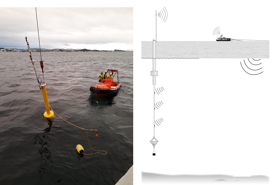
Vertical hydrophone array
The vertical array hydrophone rig, placed in the middle of the bay (Fig 2, “center bay”) consisted of a surface buoy system with hydrophones at two different depths in the water column; at 8 and 23 m depth (Fig 5). To minimize vertical movements of the hydrophones due to waves, which is a source of noise, the buoy is designed with a long slim shape to allow the waves to climb on the buoy instead of moving it up and down. The buoy was kept upright by lead weights and batteries placed in its base and by a sea anchor at the end of the hydrophone string. The buoy contains an UNO-2483G embedded computer with an internal flash drive for data-logging and instrumentation control. A radio ethernet link allowed remote control and monitoring of the system from the ship. The electronics are powered by rechargeable AGM batteries,
Bottom hydrophone rigs
Two submersible acoustic hydrophone rigs were used to record sound 8 m above bottom (Figure 6). These were placed at the inner and outer ends of the bay (“inner” and “outer” in Fig 2). Two types of hydrophones were used on these rigs; a Naxys 02345 Ethernet hydrophone and a Soundtrap 300.
An underwater housing of anodized aluminium was connected to the Naxys 02345 Ethernet hydrophone via an Ethernet cable is mounted in a steel frame. The frame is made buoyant with floats and is attached to weights (30 kg) by an 8 m rope. The underwater housing contains an Advantech UNO A157 single-board computer for data logging and system control. The computer uses a flash drive for data storage to avoid noise from the disk during logging. The electronics are powered by rechargeable A123 lithium-ion batteries with automatic low battery capacity shutdown circuitry, Logging interval, start time, gain and sampling frequency will be configured via remote control software using an Ethernet connection prior to deployment. Recorded sound data was downloaded to an external PC by using the same Ethernet connection.
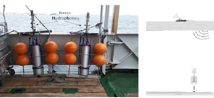
Figure 6. The two hydrophone platforms onboard HUS, ready to be deployed (left) and a figure of how it looks when deployed (right).
A sound trap 300 hydrophone was also mounted onto the abovementioned rig. These small devices (Fig 7) were used to record cod vocalisations in the area. Additionally, a depth logger was mounted together with this hydrophone.
2.6 - Placement of source and source vessel
This section describes the considerations that was made when deciding where to place the source and the vessel. We aimed at exposing the fish in the bay to the same sound exposure level (SEL) as during the seismic airgun survey. The airgun SEL`s were recorded at the three different hydrophones, placed at the same positions as the three hydrophones in the current survey, shown in Fig 2. In the airgun surveys, however, the airguns were towed along a racetrack (see Sivle et al. 2021, Fig.5), while in the current survey the source had to be kept stationary due to operational constrains. Because of this, the SEL could not be matched at all three hydrophones simultaneously. This might seem counterintuitive: if the levels at the outer hydrophone are matched, why do not the levels at the other hydrophones also match?
The following example, shown in Fig 8, illustrates what happens. For simplicity, the free surface (ghost) effect is not included; the absolute dB values are therefore not significant. In this example it is assumed that the transmission loss is simply 20*log10(distance from source).
The received level, RL, from the airgun is shown in red. It varies with range according to the assumed transmission loss. The received level at 1 meter from the airgun is marked with red ‘*’; this is the airgun source level.
The received level, RL, from the vibrator is shown in green. It varies with range according to the assumed transmission loss. The vibrator is located in a different position to the airgun and, as a result, the vibrator SL curve moves with it (Fig 8, left).
The vibrator RL curve has also been moved down in dB. This was achieved by reducing the source level of the vibrator; that is why the green ‘*’ is at a lower level than the airgun red ‘*’. This reduction in vibrator SL was done so that the RL at the outer hydrophone from the vibrator matched the value from the airgun (the curves cross at that point).
The shape of the SL curve cannot be changed: it always follows the 20*log10(distance from source). It can only be moved bodily up or down (by changing the SL) and left/right (by changing the source position).
As a result of matching the received levels at the outer hydrophone the vibrator delivers a lower, RL at the inner hydrophone. This is not because it is a different type of source: it is because it is in a different position. Therefore, the placement of the source was important; it should be placed such that the SEL was matched well at all three hydrophone locations. To estimate the range of received levels from the airguns in 2020 and 2021 we used the minimum and maximum SELs measured at the three hydrophones. To predict the levels that the vibrator would create within the bay we used a Matlab code created for the purpose by Havakustik Ltd.
The model predicted that the maximum SELs could be matched reasonably well at all hydrophones, but the minimum SELs were more difficult to match. Fig. 9 shows the predicted SEL from the vibrator at each hydrophone depending on the location of the vibrator, measured in distance to the outer hydrophone (red), compared to the minimum and maximum SELs from the airguns (black). At the ideal position, the red lines would fall exactly between the black lines for all hydrophones (a-d). However, it was impossible to match the levels at all hydrophones from the same source location. The predicted SELs for the vibrator fitted best within the measured minimum and maximum SELs from the airguns when the vibrator was placed close to the racetrack position (X=1020 m).
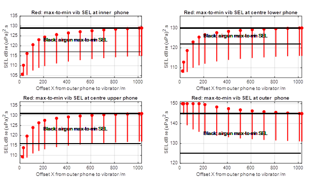
Thus, the best position for the vibrator to match the airgun SEL, was at the racetrack. However, since the ship needed to stay stationary with engines off throughout the entire experimental week, other considerations such as weather and anchoring abilities also needed to be considered, favouring positions further into the bay.
The source position thus ended up as a compromise between the best placement for transmission purposes and safety for a vessel staying at anchor with engines off, and made together by the cruise leader, project leader and the ship`s captain. This position was at a distance of about 800 m from the outer hydrophone shown in Fig. 2.
2.7 - Hydrographic observations
A SAIV SD204 sonde was used to record conductivity, temperature and pressure (CTD) data, to be able to make sound speed profiles in the area. Casts were taken at each of the three hydrophone positions and from the source ship in its anchored position (“inner”, “center”, “outer” and “source” in Fig 2). Casts were taken twice at each site, at various times throughout the week to reflect potential changes. Table 7 show the location, time and depth of the casts.
| Station number | Date | Time UTC | Latitude | Longitude | Cast depth | Comments |
| 1 | 13.02.2022 | 11:01 | 60.120133 | 5.0960333 | 75.03 | Outer hydrophone |
| 2 | 13.02.2022 | 11:10 | 60.120633 | 5.0847667 | 76.73 | Middle hydrophone |
| 3 | 13.02.2022 | 11:16 | 60.122433 | 5.0685 | 45.86 | Inner hydrophone |
| 4 | 14.02.2022 | 20:06 | 60.118592 | 5.107669 | 44.83 | Ship position |
| 5 | 16.02.2022 | 08:10 | 60.120633 | 5.0847667 | 76 | Middle hydrophone |
| 6 | 17.02.2022 | 14:30 | 60.120133 | 5.0960333 | 74.94 | Outer hydrophone |
| 7 | 17.02.2022 | 14:39 | 60.122433 | 5.0685 | 55.87 | Inner hydrophone |
| 8 | 17.02.2022 | 16:54 | 60.118592 | 5.107669 | 52.25 | Ship position |
3 - Results
3.1 - Daily Reports
Below an overview of the main activities conducted each day of the survey. All times are given as UTC.
Saturday February 12th 2022 – Mobilization in Bergen (Jekteviken). Rigging of hydrophones and sound source while in dock. Safety brief and start up meeting onboard. Dry-test on deck of sound source. Departure from Jekteviken 19:30. Wet-test of sound source in Byfjorden before transiting to Austevoll.
Sunday February 13th 2022 – Arrival at test site in Bakkasund, Austevoll around 07:00. Deployment of three hydrophone rigs in predetermined sites. CTD casts done in all three positions. Calculations and final preparations of sound exposure level based on recordings from hull mounted hydrophones during wet test. Final decision on exposure position based on weather forecast and inspection of the area. Anchor up in position and stop engines 16:07. Start first block of exposure 19:35. Finalized the first session of block number 1.
Monday February 14th 2022 – During a long silent period, the inner and outer hydrophones were taken up, data downloaded and batteries charged, and put back into position. CTD taken from ship 20:06. Successfully conducted and finished blocks 1, 2 and 3.
Tuesday February 15th 2022 – Successfully conducted block 4, 5 and 6
Wednesday February 16th 2022 – Source incident occurred during silent session (block 7.2) at 05:50. A tangled rope resulted in an accidental opening of inspection hatch at the housing of the MV BASS was flooded. Engineers/operators work on solving problems caused by this all day. Turned off the hydrophone buoy to save battery while this work was ongoing. Work finishes at 18:00 and test the source on deck. Testing went well, and source is redeployed 20:20, and continue with treatment 7.3.
Thursday February 17th 2022 – Successfully finished the last three blocks (8, 9 and 10) of the exposure plan, although with a revised version, excluding one silent session within each block to save time and finish 10 blocks as planned. CTD taken at inner and outer hydrophone positions. Retrieve the source 18:20. Retrieve the hydrophone array 20:30, and start transit toward Bergen.
Friday February 18th 2022 – Arrival in Bergen (Jekteviken). Packing and lifting off the equipment. End of survey at 12:00.
3.2 - Sound Monitoring of the marine vibrator
Sound from the BASS was recorded at three positions in the bay with Naxys hydrophones (see section 2.5). Data from deployments D1, D3, D4 and D5 in Table 5 were analysed. These represents the sound recorded in all the three positions of the bay.
The data were calibrated with a Brüel & Kjær 4229 piston calibrator with a special made coupler. The rms level for the Naxys hydrophones in the special coupler should be 148.5 dB re 1 uPa. A calibration factor was estimated for each of the hydrophones based on this.
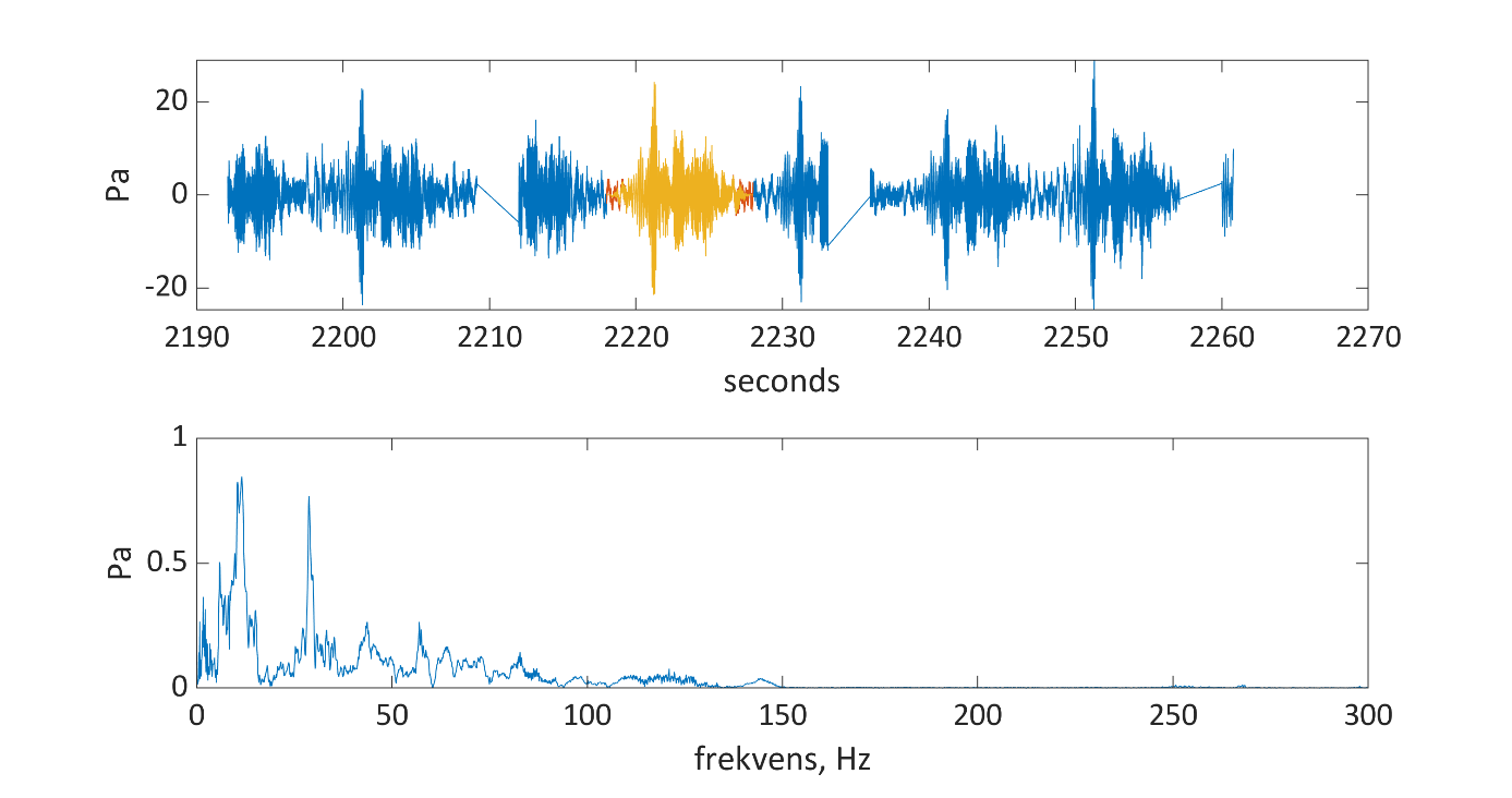
For each of the hydrophones the continuous recordings of 23 seconds long wav files with 1 s break were sorted by treatments and added into 3-hour long files for each of the treatments. The sound from the marine vibrator (se section 2.3) was continuous and consisting of a 10 s long repeated sequence of two concatenated frequency sweeps. Even though the sound was continuous the amplitude was variable as shown in Fig. 10 where about 150 seconds of recording from the hydrophone closest to the marine vibrator (D5 in table 5) are plotted. The frequency content of a 10 s long sequence shows that almost all the sound from the marine vibrator was at frequencies below 150 kHz. The data were bandpass filtered from 5 – 10000 Hz with a butterworth filter.
Sound Exposure level (SEL) was estimated both for 1 hour long periods, once for each treatment, and for 10 second long periods with 9 seconds overlap throughout each 3 hour treatment. 1 hour was used for comparison to the experiment in 2020 and 2021. The 1 hour long period was extended to compensate for the missing second in the gap between the 23 second long files. Since 1/24 seconds was missing, the period was set to 3600 s + 3600/24 + (3600/24/24)=3756 s. This means that raw data for a period of 3756 s was used for estimating SEL for one hour. SEL for 10 seconds was estimated without compensating for the 1 s long gap. This means that some of the values miss one second.
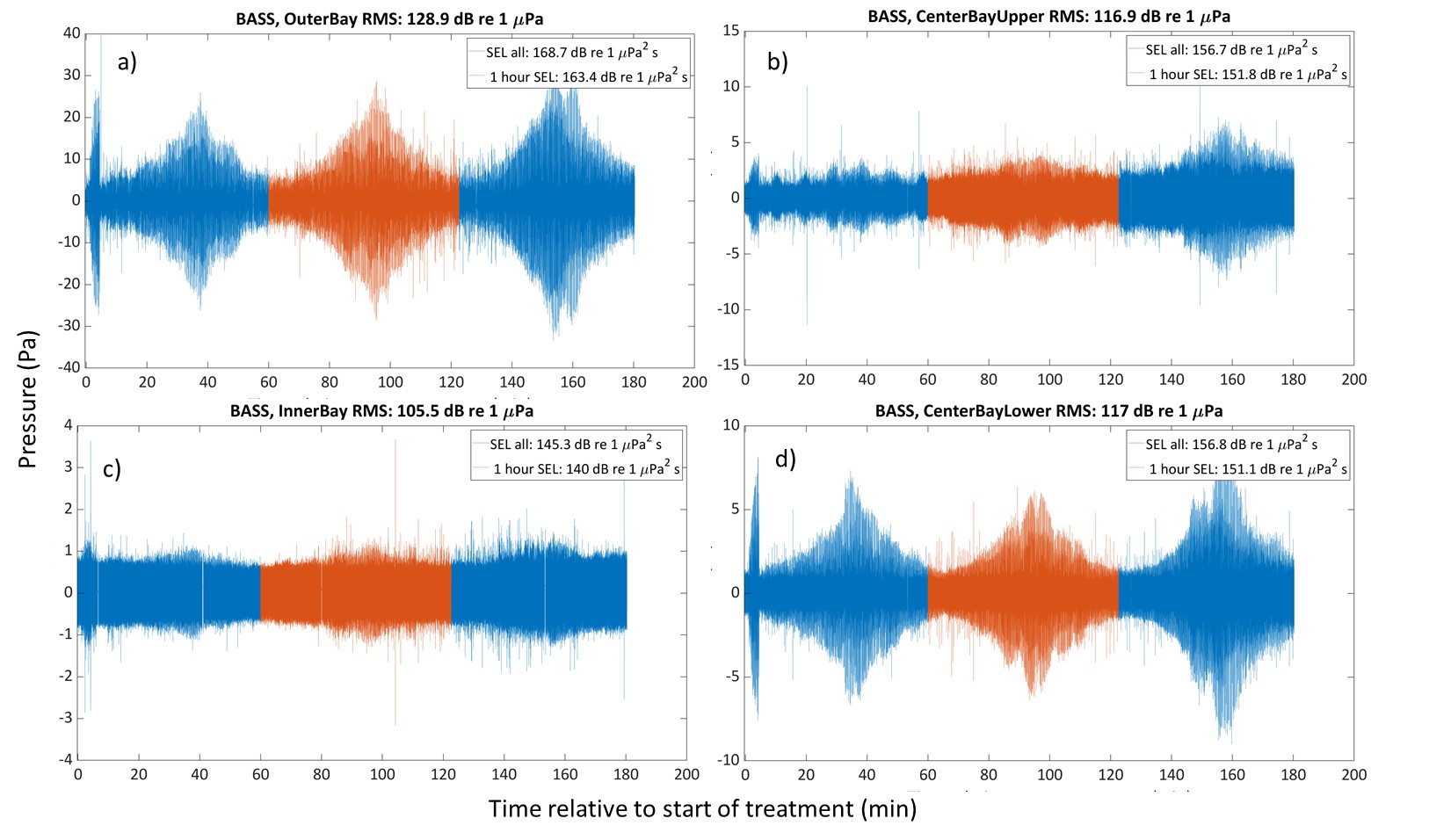
An example of recorded sound pressure data for the 3 h exposure period is shown for all three hydrophone positions in Fig. 11 where the orange part shows the data used to estimate SEL for 1 hour.
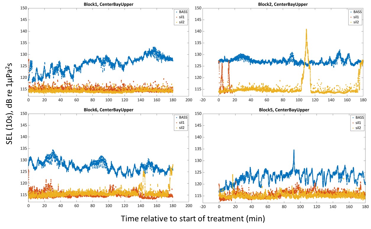
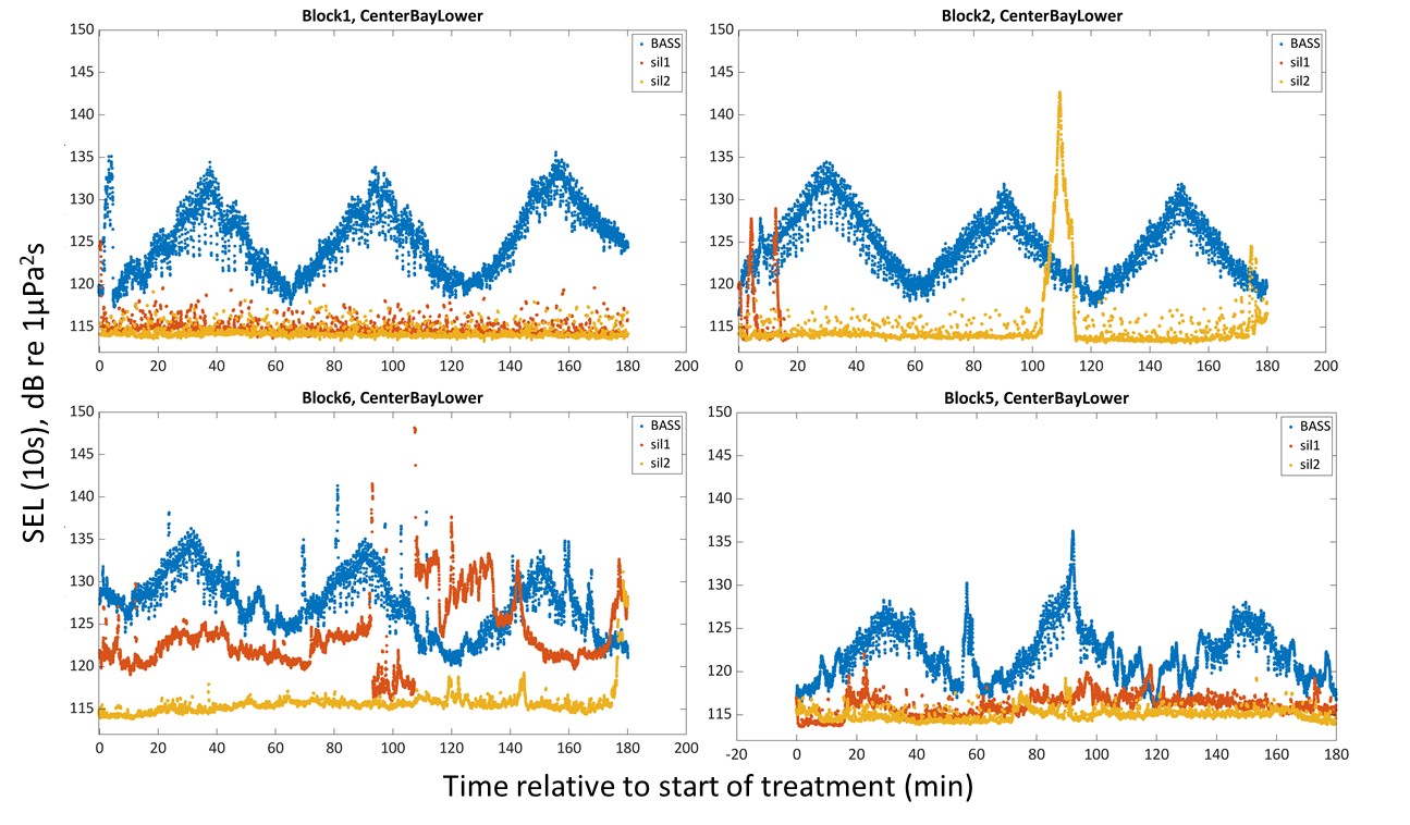
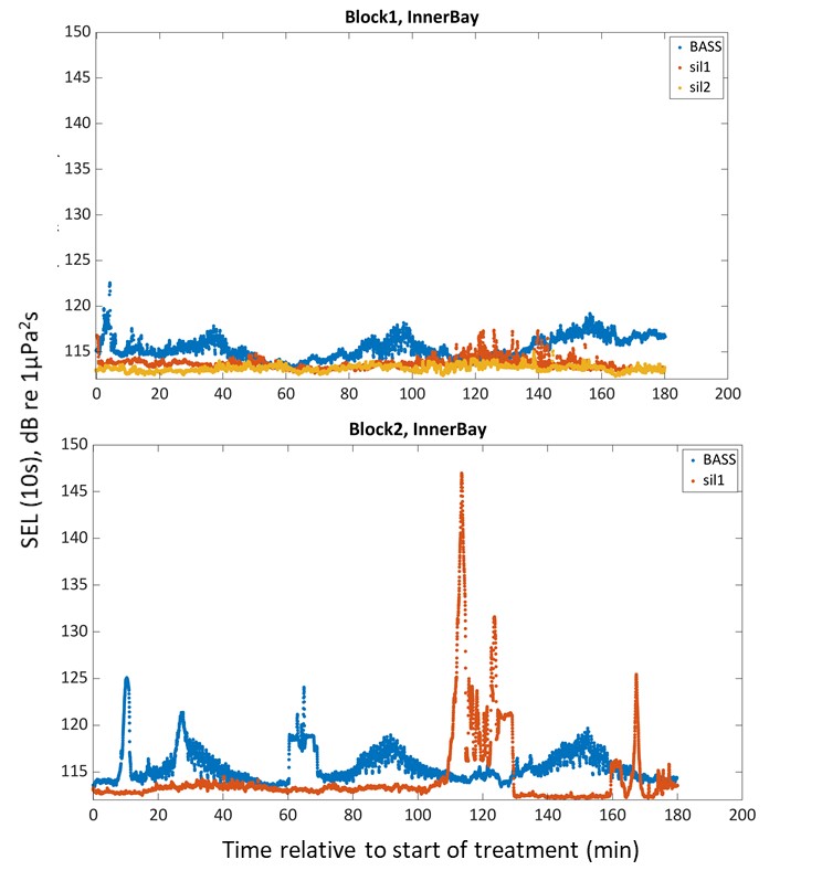
An example of the measured sound exposure levels (SEL) over a 10 sec period with 9 seconds overlap at the different hydrophones, for the different treatment (BASS and silent) types are shown in Fig. 12.
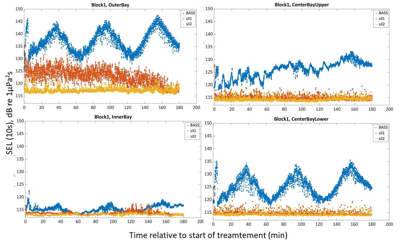
As shown in Fig. 12, the sound from the BASS exceeded the background noise (silent treatments) at all three positions.
For the outer bay, there seems to be a difference between silent 1 and silent 2, with silent 1 being more noisy than silent 2 (Fig. 12, upper left). The reason for this is not obvious, and not present at the other two hydrophones (center and inner bay), hence likely to be something local around the outer bay. Silent 2 was in the middle of the night, potentially with less human activity, so it might have been e.g. boats around during silent 1. It could not be due to differences in the weather, than it should have been present also at the other two positions.
Sound from the BASS differed between depths, as can be seen by comparing the upper and lower hydrophone of the center bay hydrophone array; in the upper part of the water column the sound is much more variable, while in the lower part, the sound from the BASS were much more like the actual transmitted sound. This may be because the upper hydrophone is closer to the wavy surface where wind and weather causes more noise, and also waves can make a variable surface reflection of the sound. Interference between the direct signal and the surface reflection could be an explanation. Measurements at different depths results in a different travel time between the direct signal and the surface reflection, so the interference will be different. According to the CTD-profile (section 3.3) the speed of sound is lower in the upper layer which also affects the sound propagation.
There was some variation between the different blocks at the same hydrophone, as can be seen in Figures 13-15. This may be due to some rotation of the anchored ship changing the angle and distance of the sound during transmission. Spikes in the background noise (silent) are likely due to boat traffic in the area.
3.2.1 - Comparing marine vibrator with seismic airgun
The BASS sound exposure level (SEL) for one hour at the outer hydrophone was very similar to the airgun SEL for one hour, even if the 10 s SEL show slightly different trends (Fig. 16, upper left), while at the inner hydrophone it is clear that the SEL for both 1 hour and 10 seconds are quite a lot lower (Fig. 16, lower left). For a full exposure cycle over 1 h, SEL was about 10 dB lower with the BASS compared to the airgun at the inner bay hydrophone. For the center bay hydrophone, the BASS also had similar, but slightly lower SEL compared to the airguns (Fig. 16, right).
Over both a 10 s period and a 3 h period, SEL was quite similar between the air gun and BASS exposure. However, an important difference was of course that the peak amplitude of the air guns is much (about 15-20 dB) higher than that of the BASS as shown in Table 8 . This is due to all the sound energy of the air gun is within a short pulse transmitted every 10 seconds, while for the BASS sound energy is spread over a 10 s period with continuous transmission. This difference; short loud pulses vs. continuous, but less loud sound, both with the same total energy, was what we aimed at testing; whether this made any difference in the behaviour of the cod. Table 8 shows a comparison of the sound from the BASS source and the 2* 40 in^3 airguns measured with the different hydrophones in the experimental bay. We compare SEL integrated over 1 hour measured in different blocks for the two methods. Gaps in the recordings are compensated for. The ambient noise and boat noise is included in the estimate. We also compare maximum values of the peak sound pressure and SEL integrated over 10 seconds for the 3 hour exposures. This illustrates that there is some variation between the repeated exposures. It also illustrates that the sound exposure level from the two different sources was most similar in the outer bay, and less similar in the inner bay. And they were also quite similar in the center of the bay. No attempts to remove the background noise from the estimates since this is a comparison of the sound the cod experienced (and not the pure sound from the sources).
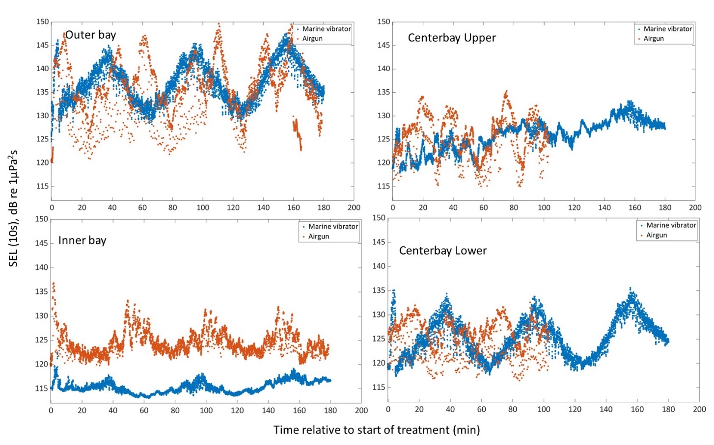
Table 8. Comparison of peak pressure and SEL for 1 s and 1 h between the BASS and the seismic airguns, for the four different hydrophones.
| BASS (block) | Seismic (block) | position | |
| SEL 1 h, dB re 1 µPa2 s | 163 (1), 164 (2), 165 (6), 166 (7) | 165(1),163 (16), 163 (17) | outer |
| SEL 10 s (max), dB re 1 uPa2 s | 148(1), 147 (2), 148 (6), 146 (7) | 150 (1), 148 (16), 147 (17) | outer |
| Peak (max), dB re µPa | 152(1), 150 (2), 150 (6), 151 (7) | 169 (1), 164 (16), 164 (17) | Outer |
| SEL 1 h, dB re 1 Pa2 s | 140 (1), 141 (2), | 150(1), 151(2), 152(4), 151 (8), 150 (9) | Inner |
| SEL 10 s (max), dB re µPa2 s | 119(1), 121 (2) | 137 (1), 135(2), 132(4), 137(8), 138(9) | Inner |
| Peak (max), dB re µPa | 126(1), 129 (2) | 145(1), 145 (2), 146 (4), 146 (8), 145 (9), | Inner |
| SEL 1 h, dB re 1 Pa2 s | 152(1), 152 (2), 152 (6) | 152(6), 155 (12) | Center upper |
| SEL 10 s (max), dB re µPa2 s | 133(1), 131(2), 134 (6) | 135(6), 137 (12), | Center upper |
| Peak (max), dB re µPa | 137(1), 136 (2), 139 (6) | 165(6), 167 (12) | Center upper |
| SEL 1 h, dB re 1 Pa2 s | 151(1), 150 (2), 154 (6) | 153(6), 153(12), | Centre lower |
| SEL 10 s (max), dB re µPa2 s | 136(1), 134 (2), 136 (6) | 132(6), 135(12) | Center lower |
| Peak (max), dB re µPa | 139(1), 135 (2), 140 (6) | 160(6), 165(12) | Center lower |
3.3 - Hydrographic observations
All results from the CTD measurements are shown in Fig. 17. Fig. 18 show the sound speed profiles for the 4 measurement stations as a function of pressure (depth). Sound speed profiles show a general upward refracting propagation condition during the entire experiment.
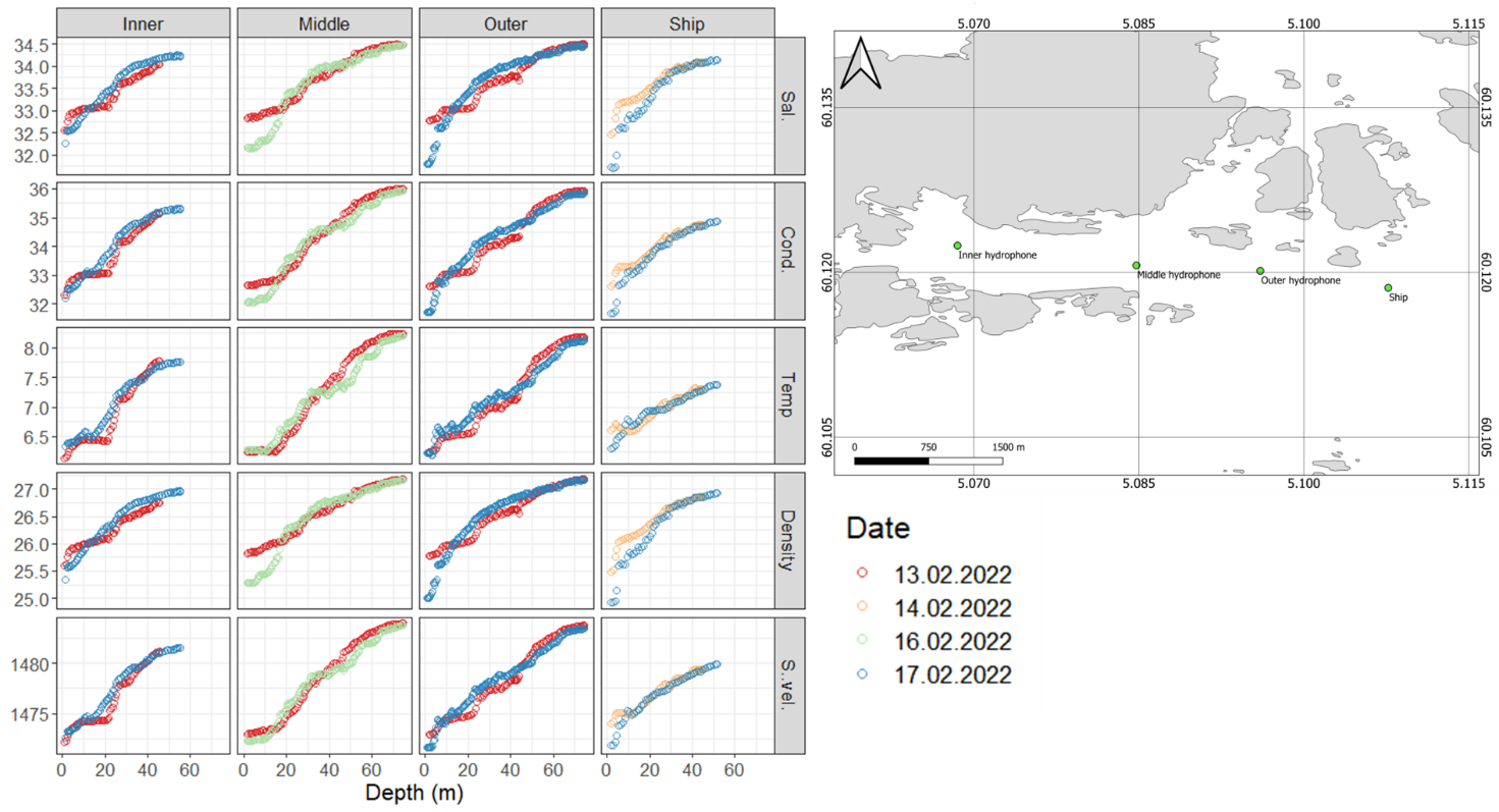
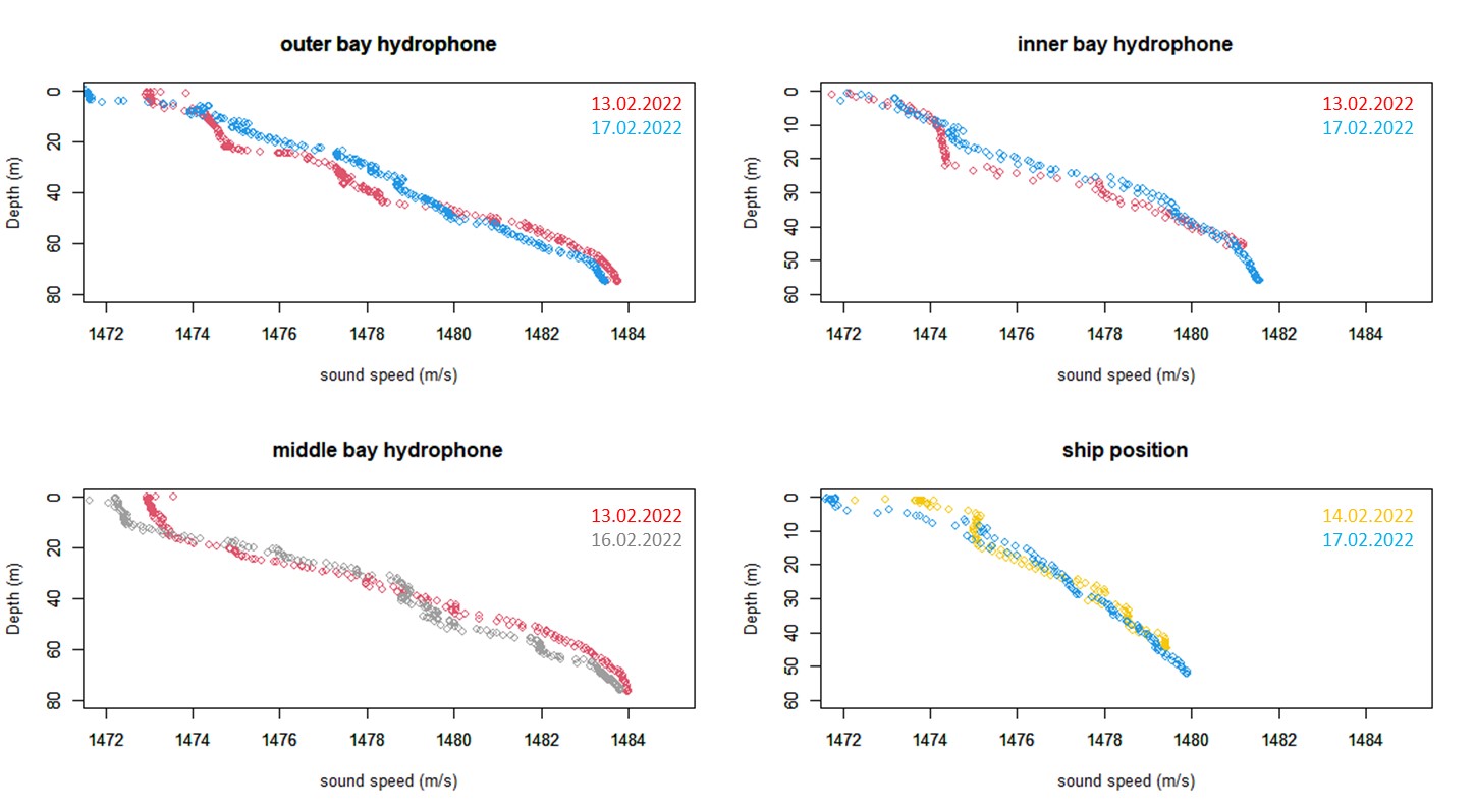
Sound speed profiles show some, but not very large variation between different days. Most variation is found in the uppermost layer. Data indicate no particular sound channels, but a general upward refrecting propagation condition.
4 - Permits
Permits to capture and tag fish and conduct experiments with sounds have been given from Fiskeridirektoratet (reference 21/16250 and 21/19313) tagging Mattilsynet (approval number 28733). The survey has been approved by IMR`s survey system (HI toktkomite). Deployment of the acoustic source and recorders are approved by the Naval Operational Headquarter.
5 - References
Sivle, L.D., Handegard, N.O. Kvadsheim, P., Forland, T.N., Ektvedt, K. W., Schuster, E., McQueen, K. (2021). Cruise report, SpawnSeis seismic exposure experiment on free ranging, spawning cod. Cruise report from surveys 2020830 and 2021826. Toktrapport/Havforskningsinstituttet/ISSN 15036294/Nr. 9–2021
McQueen, K., Meager, J., Nyqvist, D., Skjæraasen, J.E., Olsen, E.M., Karlsen, Ø., Kvadsheim, P.H., Handegard, N.H., Forland, T.N., Sivle, L.D. (2022) Spawning Atlantic cod ( Gadus morhua L.) exposed to noise from seismic airguns do not abandon their spawning site. ICES Journal of Marine Science, 10:2697-2708