Denne rapporten beskriver det femte toktet i en serie av trål-akustiske overvåkningstokt som dekker innsiget av modnende lodde til kysten av Nord-Norge. Toktet er et svar på et innspill fra næringa om å evaluere muligheten for å bruke overvåkning av gyteinnsiget på lodde til bestandsvurdering og kvoterådgivning på lodde. Tidspunktet og dekningsområdet for toktet er valgt slik at det vil være relevant å bruke til rådgivning gitt at resultatet er pålitelig. Leie av fartøy ble i år finansiert av Norges Sildesalgslag. Utvalgte områder utenfor kysten av Troms og Finnmark ble dekket ved hjelp av fiskefartøyet Vendla. Et design med stratifisert sikk-sakk transekt design ble valgt til dekningen med tilfeldig startpunkt. Ekkolodd med frekvensene 18-333 kHz ble kjørt sammen med lavfrekvent ST90 sonar, og tråling ble gjennomført på pelagiske registreringer. Loddemengden ble beregnet med 38 kHz ekkolodd. Totalbiomassen av modnende lodde ble beregnet til 274 768 tonn, med en usikkerhet beregnet til 35% (variasjonskoeffisient). Nedre 5% og øvre 95% konfidensintervall var på henholdsvis 128 879 og 448 768 tonn. Konfidensintervallet overlapper med usikkerhetsintervallet fra fremskrivingen basert på toktet høsten 2022, men er i nedre sjikt av intervallet. Lodde som ble observert i området mellom Hjelmsøy og Nordkyn dominerte estimatet (strata 3 og 4). Cirka 86% av totalbiomassen ble funnet i disse to strataene, og cirka 78% av stimene som ble observert med sonar. Sonardata viste at loddestimene i disse østlige områdene stort sett svømte i vestlig retning. Svært lite lodde ble observert i vest og i Varangerfjorden. 4 år gammel lodde (2019-årsklassen) dominerte totalt i prøvene. Gjennomsnittslengde på lodda var 16.03 cm, gjennomsnittsvekt 20.3 g og gjennomsnittlig rognprosent på 16. Det var ingen romlig trend eller trend over tid på modningen, men modningen hadde kommet lenger nær kysten enn lengre ute fra kysten. Den unormalt lave akustiske frekvensresponsen på 38 kHz som er observert for lodda i enkelte tidligere år under dette toktet, ble ikke observert i særlig grad i år. Dette er det femte året hvor estimatet fra toktet viser godt samsvar med estimatet og fremskrivningen fra høsttoktet. Dette er lovende med tanke på å bruke toktresultatene til rådgivning, men det var åpenbart at det var lodde som ikke hadde blitt dekket, særlig i russisk sone hvor de russiske fartøyene fisket hele sin kvote. Resultatene fra de fire foregående toktene ble evaluert i et ICES metoderevisjonsmøte for Barensthavslodde som ble holdt i november 2022, men rapporten fra møtet var ikke publisert i tide til utgivelsen av denne rapporten.
Testing of trawl-acoustic stock estimation of spawning capelin 2023
Report series:
Toktrapport 2023-5
ISSN: 1503-6294
Published: 12.04.2023
Cruise no.: 2023200029
Project No.: 15568-01
Research group(s):
Pelagisk fisk
,
Økosystemakustikk
,
Fangst
Subject:
Lodde – Barentshavet
Program:
Barentshavet og Polhavet
Research group leader(s):
Espen Johnsen (Pelagisk fisk) og Rolf Korneliussen (Økosystemakustikk)
Approved by:
Research Director(s):
Geir Huse
Program leader(s):
Maria Fossheim
Norsk sammendrag
1 - Summary
This report describes the fifth in a series of trawl-acoustic monitoring surveys of the maturing stock of capelin during the spawning migration to the coast. The survey is a response to a proposal from the industry to evaluate the possibility of using winter monitoring of maturing capelin as an input to the capelin assessment and advice. The timing and geographic coverage of the survey are such that they would be relevant to use for advice given that the output is reliable. The rental of the vessel was this year funded by the Norwegian Fishermen’s Sales Organization for Pelagic Fish. Pre-defined areas off the Troms and Finnmark coast were covered using FV Vendla. A stratified random transect design was adopted with a zig-zag transect grid covered in west-east direction over 6 strata. Echo sounders with frequencies from 18-333 kHz were run together with a low frequency ST90 sonar, and target trawls were carried out on significant pelagic aggregations. Capelin abundance was estimated using 38 kHz data. The total biomass of maturing capelin in the coverage area was estimated at 274 732 tons, with a CV of 35%. The 5% lower and 95% upper confidence limits were 128 879 and 448 768 tons, respectively. The confidence bands overlap with the uncertainty intervals in the prediction from the autumn 2022, but on the low side. Capelin recorded in the stratum covering the coast from Hjelmsøy to Nordkyn dominated in the estimate (strata 3 and 4). Ca. 86% of the total biomass was found in these two strata, and ca. 78% of the schools detected with sonar. Sonar data showed that the capelin schools in these easterly areas in general moved in a westerly direction. Very little capelin was recorded in the west and in the Varangerfjord. Age 4 capelin (2019 year class) totally dominated the sampled capelin. Mean length of the capelin was 16.03 cm, mean weight 20.3 g, and mean roe percentage was 16 with no temporal or geographical trend, but maturation had extended further close to the coast than off the coast. The abnormal low frequency response at 38 kHz observed in some of the earlier survey years, was not observed to any large extent this year. This is the fifth year that the estimate from this survey shows consistency with the estimate from the autumn survey. This is promising for the use of the survey results for advice, but it was obvious that there were maturing capelin that had not been covered, in particular in the Russian EEZ where the Russian vessels were fishing. The results from the 4 previous survey years were evaluated in a recent ICES capelin benchmark meeting in November last year, but the report from the meeting was not published by the time of the release of the present report.
2 - Introduction
In 2018, there was a proposal from the industry forwarded through FUR (‘Faglig Utvalg for Ressursforskning’; Joint science/industry association for resource investigations), that funding from the Fisheries Resource Tax (FFA) should be spent on a winter monitoring of the Barents Sea capelin spawning migration to evaluate whether such monitoring could be used to improve capelin assessment and quota advice.
The main spawning of the Barents Sea capelin takes place in the period from late February to early April mainly along the coast of northern Norway between Tromsø and Varangerfjord, but also along the coast in north-west Russia. If there is opening for a fishery, it takes place on maturing capelin off the spawning areas. The fishery is open from late January, but typically starts in late February. In the present assessment of the Barents Sea capelin stock, there is only one annual input to estimate the biomass of the maturing stock, and that is the trawl-acoustic data from the joint Russian/Norwegian Barents Sea monitoring in the autumn (ICES, 2020). The quota advice is based on a forward projection of maturing capelin biomass from the autumn survey the previous year to 1 April the present year, including associated uncertainty (Gjøsæter et al., 2002). Previous attempts have shown that winter monitoring of the capelin spawning migration is challenging (Ref: https://www.hi.no/resources/images/3_arig_rapport_gyteinnsig_lodde.pdf), both because the spawning locations span a wide geographical range and because the timing of the migration and hence availability to acoustic detection, is variable. Based on this, the survey estimate must be understood as a minimum estimate of the spawning stock. Nevertheless, a reliable winter survey could potentially reduce uncertainty in the assessment of biomass of maturing capelin and improve the advice. IMR therefore approved the proposal from the industry and took on to conduct a series of three winter monitoring surveys which were carried out from 2019 to 2021 which was extended with a fourth year in 2022. Here we report the results from the fifth year in the series and the second year that the fishery has been open during the survey period.
2.1 - Objectives
The main objective of this effort is to conduct a series of surveys with a timing and a design such that it could potentially have been used in an advice process. The surveys will form the main basis for an evaluation of the usefulness of such a monitoring in capelin assessment and advice.
3 - Methodology
3.1 - Vessel
The fishing vessel FV Vendla was selected to carry out the acoustic survey, which started in Tromsø on 26 February and ended in Kirkenes on 9 March.
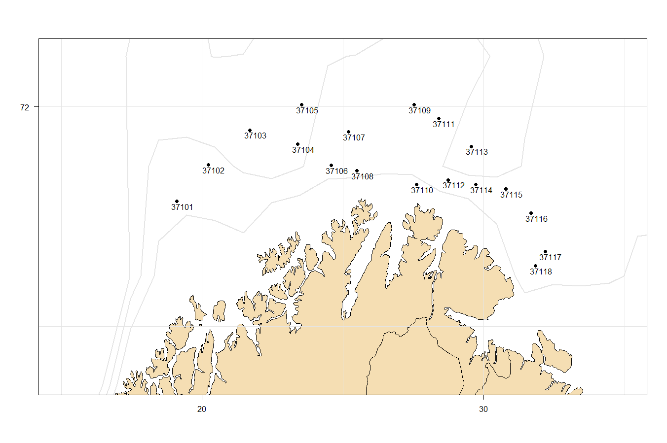
3.1.1 - Survey design
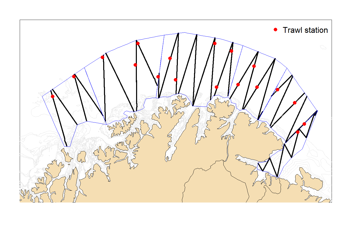
We adopted a stratified random transect survey design with the allocation of effort reflecting the expected abundance of capelin within a given stratum. The strata and distribution of effort are shown in Figure 1. The coverage area and design are similar to the design used from 2019-2022 (see survey reports for details, available at https://www.hi.no/resources/Toktrapport-loddetokt-mars-2019.pdf , https://www.hi.no/hi/publikasjoner/toktrapporter/2020/testing-of-trawl-acoustic-stock-estimation-of-spawning-capelin-2020-nr.-2-2020 and Survey-report-capelin-spawning-survey-2021_final-1.pdf (hi.no) and Testing of trawl-acoustic stock estimation of spawning capelin 2022 | Havforskningsinstituttet (hi.no) for the years 2019-2022). It is important to underline that the survey area we have defined is a core area for the capelin spawning migration, and the survey period is adequate in the case an advice would have been provided, but this is not a complete coverage of the Barents Sea capelin spawning stock.
Like in 2019-2022, we implemented a zig-zag transect design, which has the advantage of allowing more time spent on transects and less on transit compared to a design with parallel transects. In 2020-2022, we adopted a design including a complementary return zig-zag going in the opposite direction, but there was not enough available survey time to do the same this year. With one vessel available for 11 days we aimed for a single coverage.
Some information on capelin distribution was available from the capelin fishery, the NSS-herring survey and from fish plants reporting the presence of capelin in cod stomachs, and based on this information, we allocated more effort into stratum 3 where capelin had been fished and less in strata 1 and 2 where little capelin had been observed.
Strata boundaries were drawn using the software Stox (Johnsen et al., 2019), and allocation of effort within the strata was done using the “survey planner” function in the R package Rstox ( https://github.com/arnejohannesholmin/sonR). The method used for generating the zig-zag transect plan was “Rectangular enclosure zigzag sampler” (Harbitz, 2019) in strata 1-5 and ‘Equal space zigzag sampler’ in stratum 6 (Strindberg and Buckland, 2004). The starting point of the transects was random in all strata.
3.2 - Acoustic data collection and processing
3.2.1 - Echo sounder
Acoustic data from calibrated Simrad EK80 echo sounders were collected at frequencies of 18, 38, 70, 120, 200 and 333 kHz on board Vendla. Transducers were mounted in a drop keel 3 m below the vessel hull. Data were collected up to 500 m range and with a ping interval of about 1 second. Raw acoustic data were scrutinized daily using the LSSS software at 38 kHz to the categories ‘Capelin’, ‘Herring’, ‘Bottom fish’ and ‘Other’. The scrutinized data were stored at a resolution of 0.1 nmi horizontal and 5 m vertical and exported in units of Nautical Area Scattering Coefficient (NASC; m2nmi-2). This output was used for the biomass estimation (see section below).
3.2.2 - Sonar - data collection and processing
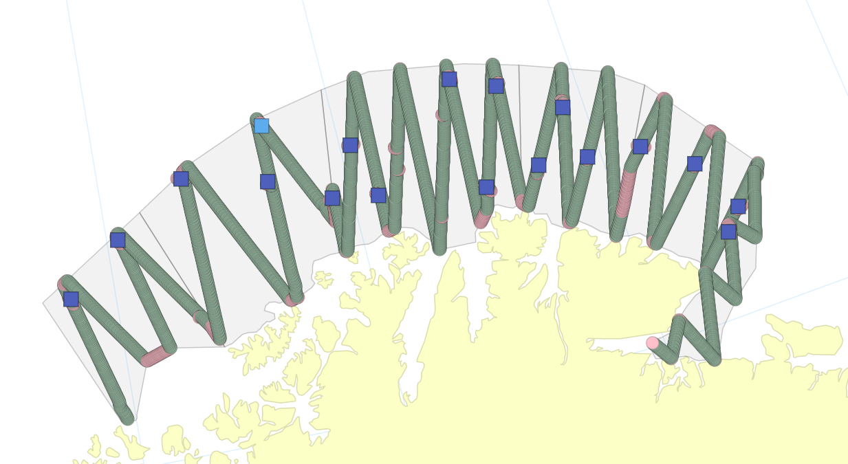
Sonar data were collected continuously using a Simrad ST90 low frequency sonar. The settings used for data collection are given in Table A1 in the Appendix. The sonar data were processed onboard during the survey using the LSSS module PROFOS (Peña et al., 2013). The settings used for school detection (school growing) are listed below:
-
Select a short period with good school registrations.
-
Choose a few schools and test with manual growing what the school properties are, including minimum size, number of pings, number of missing pings, Sv threshold.
-
Test that automatic growing works.
-
In periods with clear schools, run automatic growing.
-
Merge schools that have several school boxes and delete false schools.
The lower threshold for size was varied between 1500 - 5000 m2 depending on the background noise levels. Some of the smallest schools were thereby not included in the analyses. In some periods many small schools were observed, and it was difficult to extract all the schools (Figure A1 in Appendix), again leading to some of the smallest schools being excluded. The other settings used for data processing were kept the same for all data (See Table A2 in appendix for list of settings).
3.2.3 - Sonar - data analyses
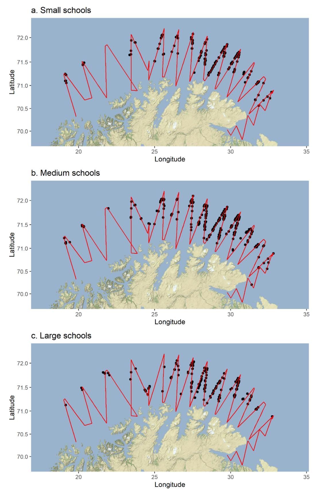
A threshold for smallest acceptable school size was set to 5000 m2 and the minimum number of pings per school was set to 30 pings. The schools were further divided into small (25th quantile of all school sizes and smaller), medium (25th – 75th quantile of all school sizes) and large (75th quantile of all school sizes and larger).
The Profos software calculates average values for school depth, area, volume backscattering strength (Sv in dB re m-1), swimming direction and speed. School depth in the horizontal beams is calculated from the tilt angle of the beams and range to school. As the beam tilt angle was adjusted to fit the general depth of the schools and not adjusted for individual schools this gives quite a rough estimate of school depth. School speed and direction are based on the first and last detection of a school. School area is based on the sum of the samples of the school per ping and then averaged for the per school results . The sonar was not calibrated and the volume backscattering values (Sv in dB re m-1) are relative.
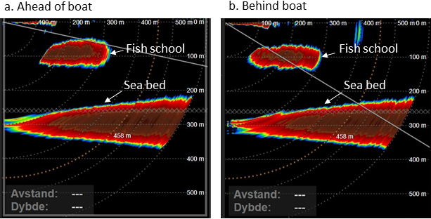
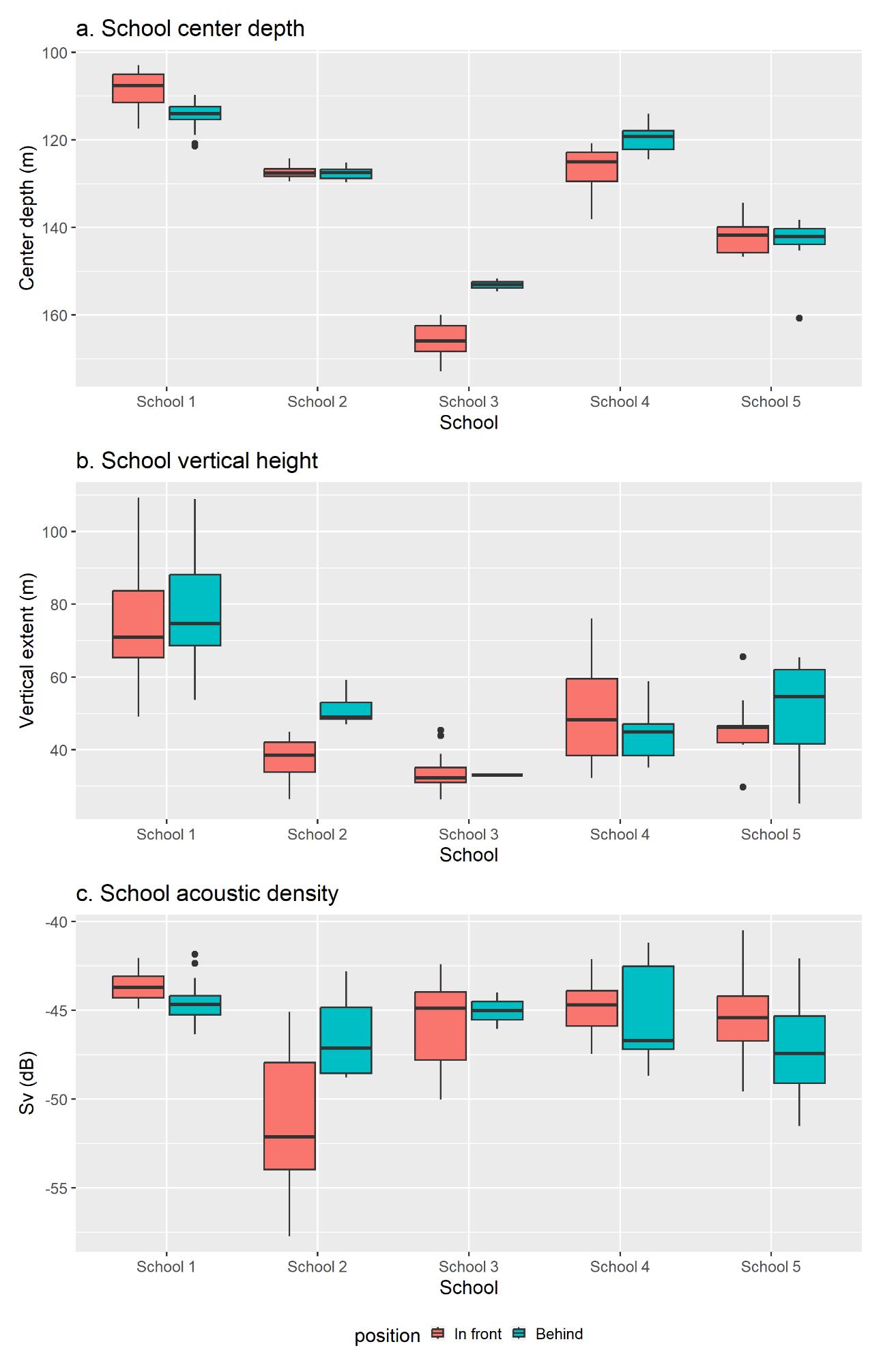
School avoidance was investigated in 5 schools. Each school was first monitored in front of the vessel at 100 – 400 m distance. As the vessel passed over the school the vertical sector was moved to 270° pointing behind the vessel and the same school was monitored 100 – 400 m behind the vessel (Figure A2 in the Appendix). The average depth, vertical height and Sv values before and after passing over with the vessel were compared.
The search radius was 1500 but increased at times to monitor schools further away from the vessel. Schools beyond 1500 m radius or schools detected when moving out of the transect lines for trawling have not been removed from the data.
3.3 - Biological sampling
A Multpelt trawl was applied for biological sampling. Two splits in the codend were made to protect the trawl and avoid large catches.
Only target trawl hauls were carried out, i.e. on significant pelagic aggregations that were thought to be capelin. From every trawl haul, a maximum of 100 randomly selected capelin were sampled. Weight and length were measured for all, while age, sex and gonad stage were sampled for 50. In addition, roe weight was measured per specimen for the 50 individuals, but the scale was not precise enough to allow for quality measurements at such a fine scale so the weight of roe for all females among the 50 at each individual station was summed up and recorded. By dividing this roe weight with total weight of the females, roe percentage could be calculated. In addition, individual length and weight of other species were recorded when they were found in the sample.
3.4 - Biomass estimation
The Stox 3.6.0 application (Johnsen et al., 2019) was used to calculate a standard transect-based trawl acoustic estimate. Some main steps of the protocol can be mentioned: All acoustic recordings outside the transects (due to for instance trawling) were excluded from the estimation. All the assigned biological stations were given equal weight when generating the total length distribution used in the estimation. The following target strength – length relationship was applied for the density (numbers/nmi2) calculation (Dommasnes and Røttingen, 1985):

Abundance of fish in numbers and biomass were estimated by stratum and age based on 2000 bootstrapping iterations of biotic stations and acoustic transects. The results are reported in Tables 1 to 3.
4 - Results
4.1 - Capelin biomass estimate
An overview of all transects and stations included in the biomass estimation is shown in Figure 2. The total biomass of maturing capelin within the coverage area was estimated to 274 732 tons (Table 1), with a relative sampling error or Coefficient of Variation (CV) of 35% (Table 1). This CV is based on bootstrapping with replacement of transects as well as bootstrapping of biological stations used in the assignment. A 5% lower and 95% upper confidence limit were calculated from 2000 bootstrap replicates, and the lower and upper limits were 128 879 and 448 768 tons, respectively. Estimates of abundance by age with associated CV are provided in Table 2. Fish of age 4 (2019 year class) was dominant. The 2019 year class also dominated the samples in the spawning survey in 2022. Mean length and weight by age are given in Table 3. The confidence interval of the estimate is overlapping with the uncertainty interval of the prediction from the 2022 autumn survey. The highest biomass estimates were from strata 3 and 4 (Table 1).
| Stratum | 5th percentile | Median | 95th percentile | Mean | CV |
|---|---|---|---|---|---|
| 1 | 425 | 1172 | 2098 | 1176 | 0.43 |
| 2 | 638 | 1447 | 2540 | 1459 | 0.43 |
| 3 | 29775 | 149645 | 325941 | 160448 | 0.56 |
| 4 | 33478 | 75934 | 121214 | 76182 | 0.34 |
| 5 | 6469 | 34461 | 82426 | 35027 | 0.66 |
| 6 | 8 | 422 | 1038 | 440 | 0.76 |
| Survey | 128879 | 266761 | 448768 | 274732 | 0.35 |
| Age | 5th percentile | Median | 95th percentile | Mean | CV | |
|---|---|---|---|---|---|---|
| 3 | 4197 | 9598 | 17941 | 10079 | 0.42 | |
| 4 | 63810 | 127548 | 215021 | 131529 | 0.35 | |
| 5 | 2312 | 6282 | 12153 | 6660 | 0.46 | |
| 6 | 248 | 1489 | 3351 | 1623 | 0.60 | |
| Age | Mean weight (g) | CV weight | Mean length (cm) | CV length |
|---|---|---|---|---|
| 3 | 15.64 | 0.03 | 15.2 | 0.006 |
| 4 | 20.76 | 0.01 | 16.3 | 0.003 |
| 5 | 24.71 | 0.04 | 17.0 | 0.007 |
4.2 - Acoustic recordings
4.2.1 - Echo sounder
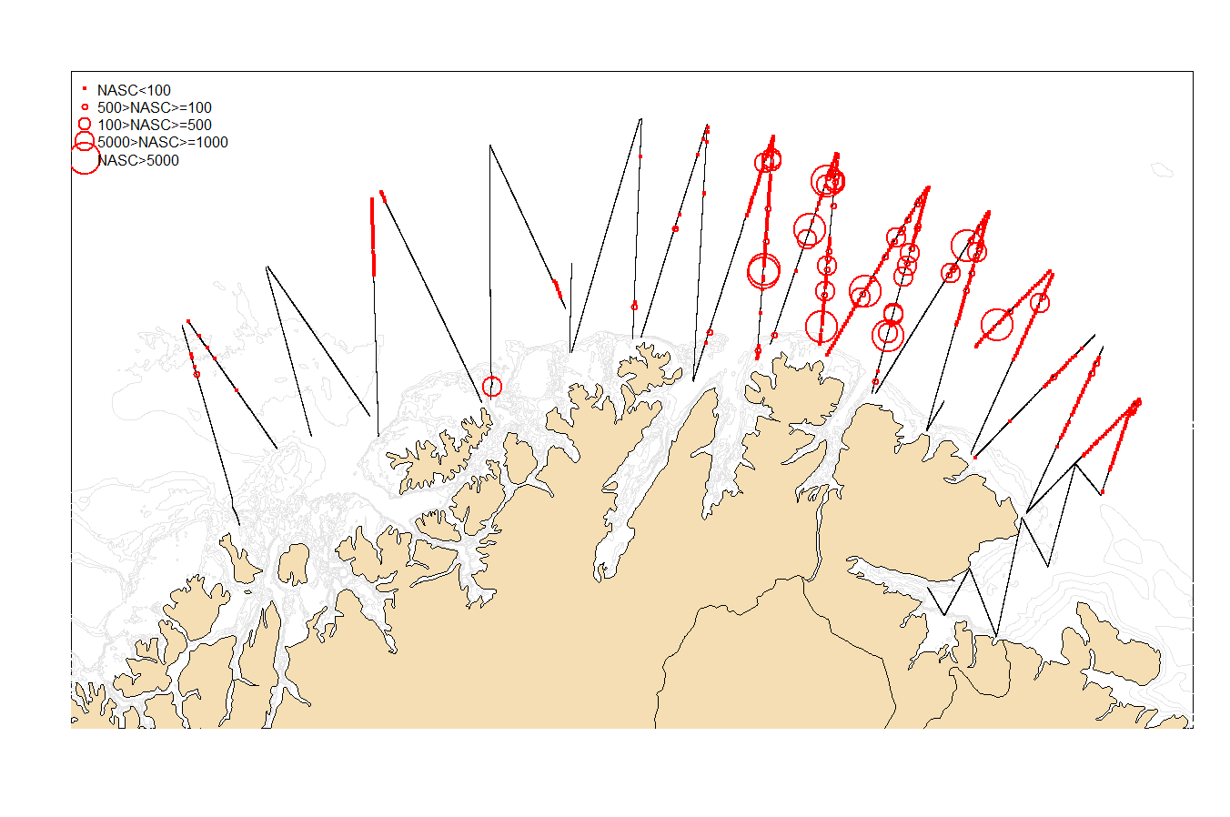
The distribution of acoustic backscatter allocated to capelin is shown in Figure 3. Echo sounder recordings from the coastal shelf area north of Varangerhalvøya dominated the echo sounder recordings. There were lower capelin recordings in the western coverage area.
4.2.2 - Sonar
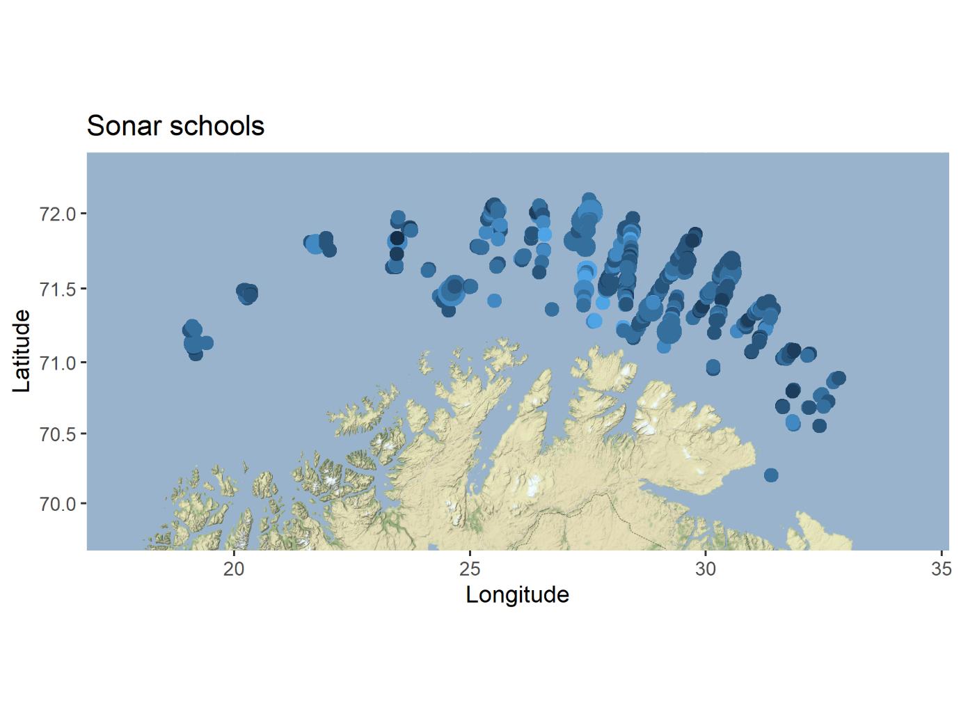
During the survey 736 schools were detected and extracted based on the sonar data and analyzed. Most schools were detected in stratum 3 and 4 and were mainly in the outer areas of transects (Table 4, Figure 4 and Figure A3 in the Appendix).
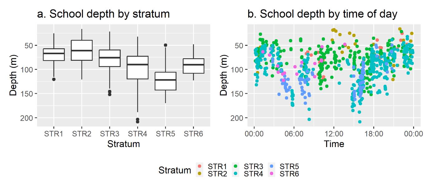
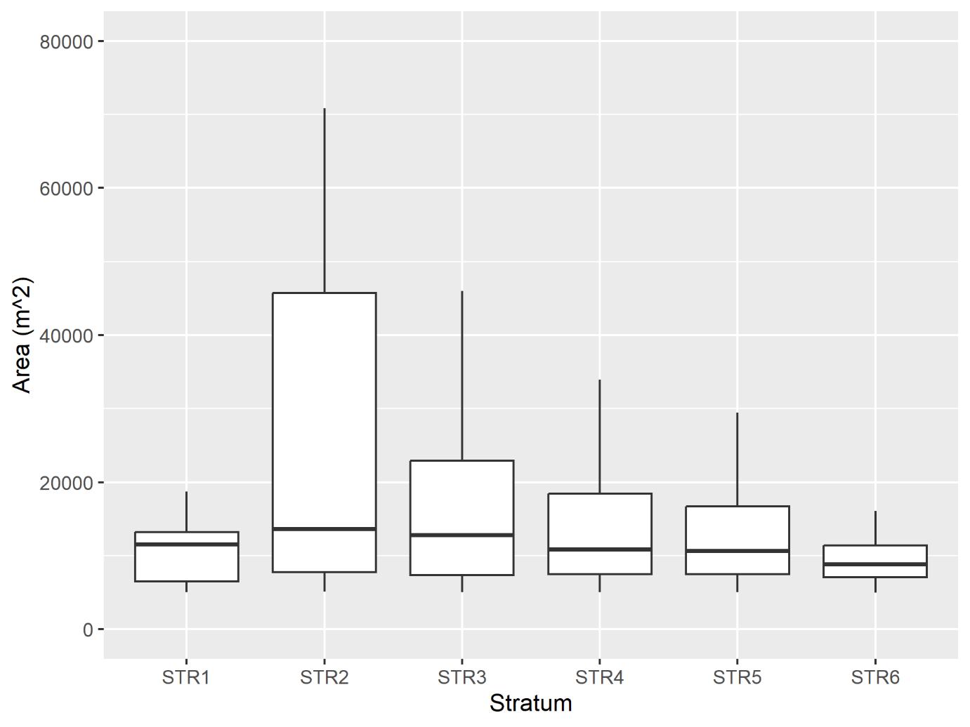
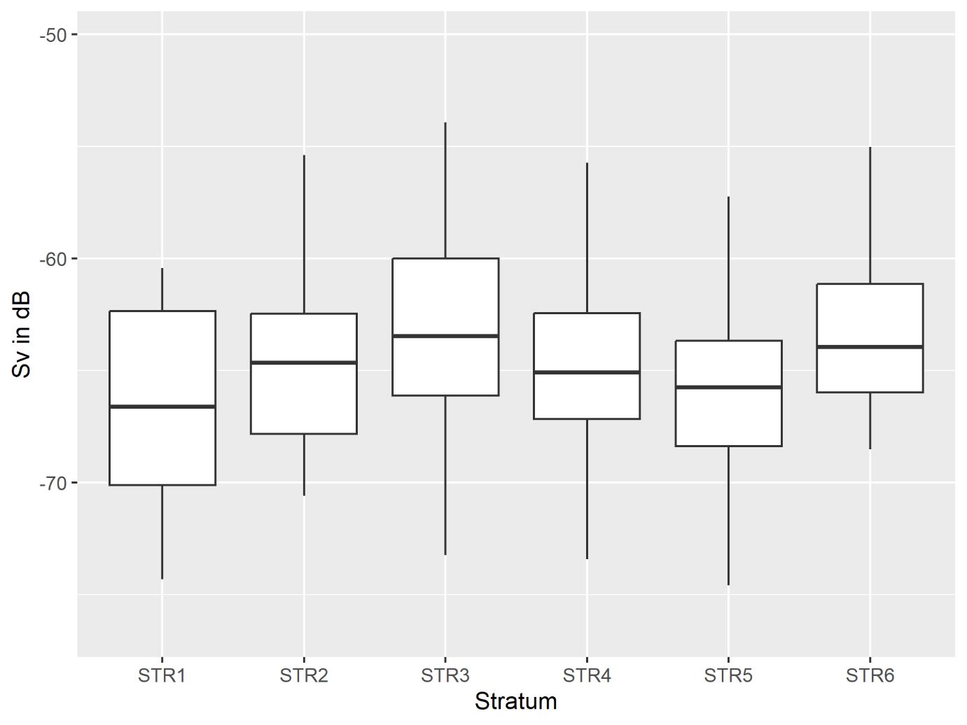
School area was mainly between 8000 and 20 000 m2 (Figure A4 in the Appendix). Average school Sv values ranged mainly between -60 and -70 dB (non-calibrated values), with no significant differences between strata (Figure A5 in the Appendix). School depth was mainly shallower than 100 m in strata 1- 3 and slightly deeper in strata 3 and 4, down to 150 m depth (Figure 5a). The schools in strata 3 and 4 were distributed deeper early in the morning (6 – 8 am UTC) and early in the evening (3 – 5 pm UTC; Figure 5b). More accurate school depth can be obtained from the vertical beams. However, it was not feasible to scrutinize both the horizontal and vertical beams during the survey. Scrutinizing the horizontal data took about 4 h per 24 h of data.
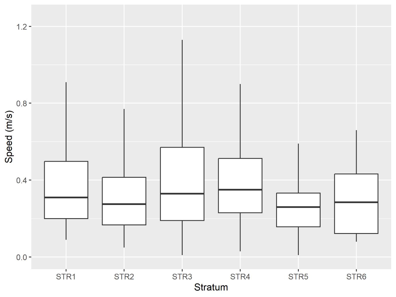
School speed varied mainly between 0.1 and 0.6 m s-1 (Figure A6 in the Appendix). For better estimates of swimming speed, the ping-to-ping data should be analyzed and ideally take account of current speed and direction. A strong current (0.7 kts) was for instance present in stratum 5 that will influence swimming speed.
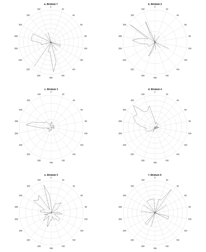
School swimming direction was consistent in strata 3 and 4 with a westerly direction in stratum 3 and a westerly/northwesterly direction in stratum 4 (Figure 6). School swimming directions in strata 1 – 2 and 5 – 6 were more variable.
5 schools were investigated for possible vessel avoidance. No clear and consistent differences in average school depth, vertical height and volume backscattering strength were detected before compared to after passing over the school. However, the vertical extent and acoustic density (Sv in dB re 1m-1) increased in school 2 as the vessel passed. Some small changes in school depth were also observed in some of the schools, the changes were 10 – 20 m.
| Stratum 1 | Stratum 2 | Stratum 3 | Stratum 4 | Stratum 5 | Stratum 6 | |
| No. Schools | 24 | 34 | 241 | 333 | 89 | 16 |
| No. Small | 8 | 6 | 59 | 81 | 22 | 5 |
| No. Medium | 13 | 11 | 104 | 181 | 52 | 10 |
| No. Large | 3 | 17 | 78 | 71 | 15 | 1 |
| Average (sd) depth (m) | 71 (23) | 60 (29) | 79 (25) | 98 (34) | 121 (27) | 89 (22) |
| School average heading | 223° | 240° | 226° | 261° | 216° | 186° |
4.3 - Biology of the capelin
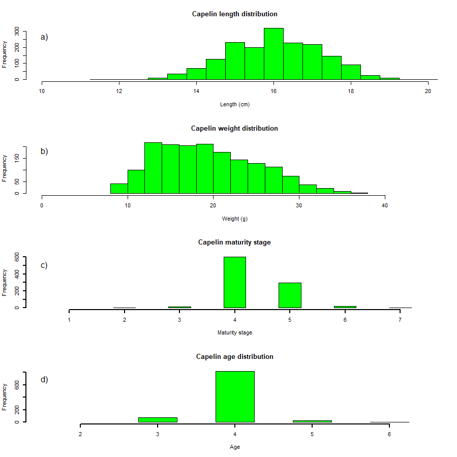
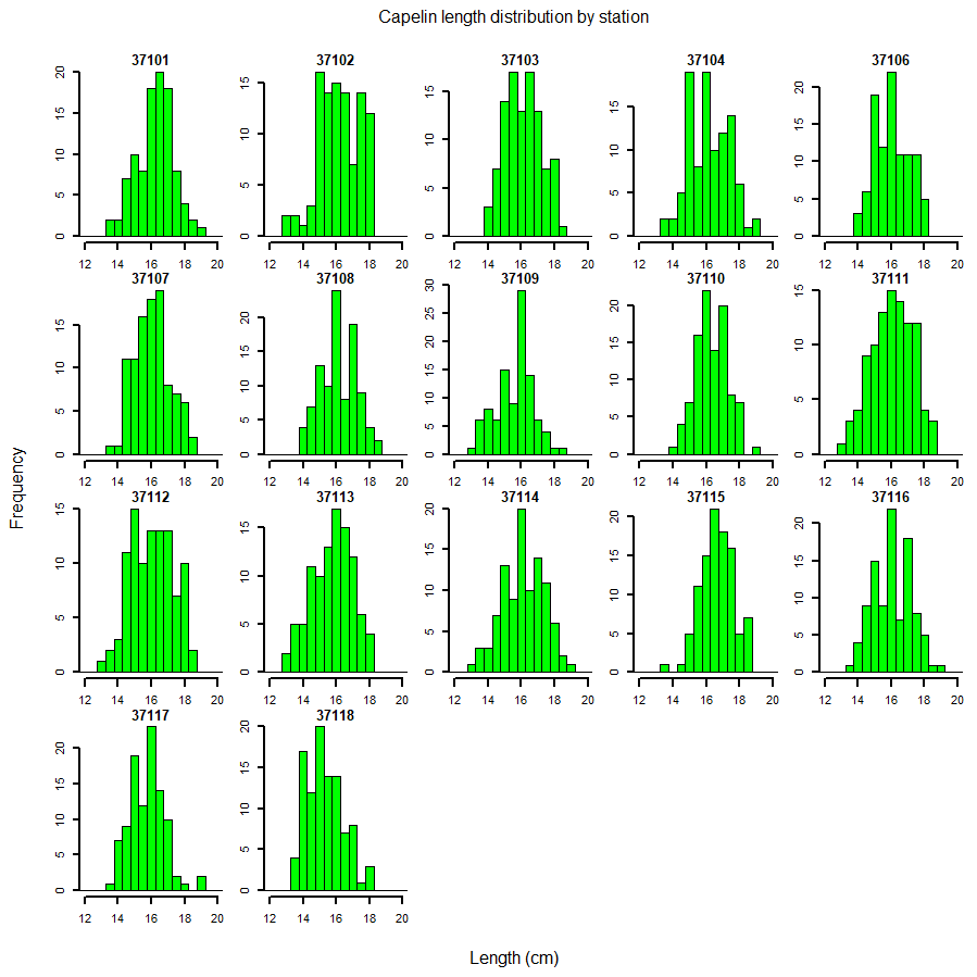
The mean length of capelin based on all biological samples was 16.03 cm (Figure 7). The length distribution supports the assumption in the stock prediction that capelin >14 cm are migrating to the coast to spawn. Length distributions by station are presented in Figure A9 in the Appendix. Mean weight was 20.3 g (Figure 7). Most of the capelin was in spawning stage 4, which is maturing, and age 4 capelin totally dominated in the samples.
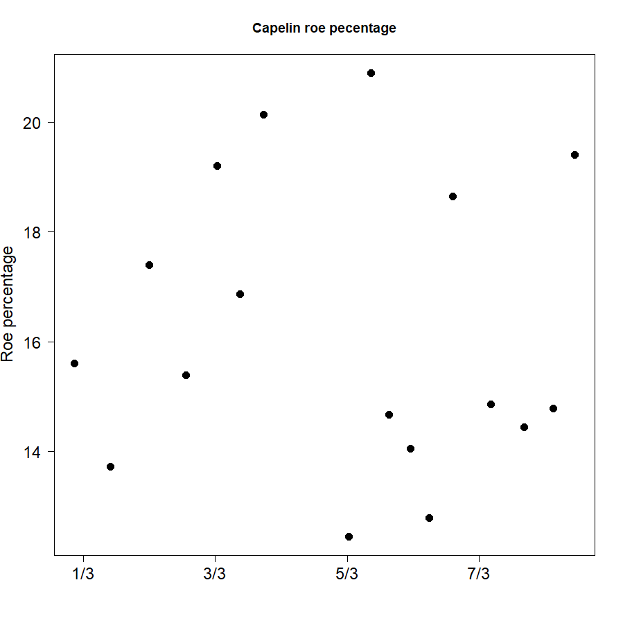
The roe percentage was calculated to get additional information on the maturation and spawning progress. It is calculated as the sum weight of roe in the individual samples divided by the total weight of females in the same sample. The results are presented in Figure 8. Roe percentage varied between 12 and 22. There was no obvious trend over time or from west to east, but maturation had typically progressed less off the coast than closer to the coast.
No Norwegian spring spawning herring were observed in the survey area.
5 - Concluding remarks about the survey
The total biomass was estimated at 274 732 t, with a sampling variance expressed as Coefficient of Variation (CV) of 35%.
The dominating amounts of capelin were found in the east between Hjelmsøy and Nordkyn. Very little capelin was recorded in the west and in the Varangerfjord.
This is the fifth year of conducting this survey and like for previous years the survey result overlaps with the lower range of the confidence band of the stock forecast based on the autumn survey. The consistency in results despite the dynamics of the migration is promising for the use of such monitoring for advice purposes, but it is also obvious that a significant proportion of the maturing capelin is not covered, in particular in the east. This year the Russian fleet was fishing their entire quota in REEZ which was not covered by the survey.
The results from the four previous years of this survey series were presented for the 2022 ICES capelin benchmark meeting and its usefulness for the capelin advice was evaluated there. The report from that meeting will be published shortly.
6 - Acknowledgments
The skipper and crew of FV Vendla are thanked for their excellent assistance and engagement during the whole survey. The costs for vessel rental were covered by the Norwegian Fishermen's Sales Organization for Pelagic Fish .
7 - Appendix
7.1 - Sonar
7.1.1 - Background
Low frequency omni directional fisheries sonar (i.e. 14-24 kHz) are used by fishermen for long distance search of commercial fish aggregations. During surveying, the large sampling volume of the sonar can provide valuable information of the spatial distribution of fish schools. In particular, this can be important if there are few schools and they have a patchy distribution. The sonar can also provide valuable information about potential vessel avoidance or schools distributed shallowly in the echo sounder surface dead-zone.
Also, when schools are tracked at low vessel speed or for a long period, the direction and speed of the schools can be estimated, information that is particularly important for the capelin during the spawning migration towards the coast.
Sonar data from Simrad ST90 at a frequency of 20 kHz was collected continuously with horizontal beams up to 1500 m range with a tilt of -3 deg when surveying. The tilt was adjusted up to -10 deg in some areas when schools were distributed deeper. Vertical beams were set across vessel track direction with a range of 600 m. Outside the survey transects, the tilt and range were adjusted to ensure a better sampling of the schools either for detailed inspection or during trawling.
The ST90 sonar of Vendla was not calibrated prior the start of the survey, but was calibrated prior to the survey in 2021 following the methodology proposed by Macaulay et al. (2016).
On some occasions, but not consistently, schools that were observed with the sonar outside of the transect were inspected with sonar and echo sounder at closer range, and sometimes followed by a trawl haul for biological sampling. The survey was then resumed at the point the transect was left.
7.1.2 - Data collection and processing
-
Range 1500 Tilt 3 - 10° Tilt was adjusted depending on school depths Bandwidth 0.5 kHz Beam vertical Narrow Beam form LFM Noise filter Off Table A1. Sonar settings used during surveying.
| Adaptive threshold (dB) | 12 |
| Maximum allowed missing pings | 1 |
| MinMaxDeltaSv | 2 |
| Minimum area (m2) | 1500 – 5000 |
| Maximum area (m2) | 1000000 |
| Maximum aspect ratio | 15-20 |
| Minimum number of consequent pings | 7 |
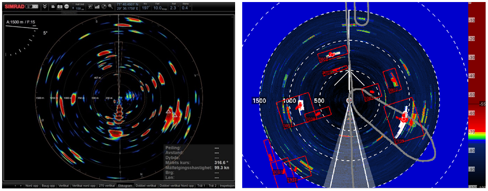 Figure A1. Example of a situation where a large number of small schools are detected with the sonar. To the left is a screen dump from the sonar and to the right from PROFOS (LSSS).
7.1.3 - Results
7.2 - Biological samples
8 - References
Dommasnes, A., and Røttingen, I. 1985. Acoustic stock measurements of the Barents Sea capelin 1972-1984. In The Proceedings from the Soviet-Norwegian symposium on the Barents Sea capelin, pp. 45-108. Ed. by H. Gjøsæter. Institute of Marine Research, Bergen, Norway.
Gjøsæter, H., Bogstad, B., and Tjelmeland, S. 2002. Assessment methodology for Barents Sea capelin, Mallotus villosus (Müller). ICES Journal of Marine Science, 59: 1086-1095.
Harbitz, A. 2019. A zigzag survey design for continuous transect sampling with guaranteed equal coverage probability. Fisheries Research, 213: 151-159.
ICES 2020. Arctic Fisheries Working Group (AFWG). ICES Scientific Reports. 2:52. 577 pp. http://doi.org/10.17895/ices.pub.6050
Johnsen, E., Totland, A., Skålevik, Å., Holmin, A. J., Dingsør, G. E., Fuglebakk, E., and Handegard, N. O. 2019. StoX: An open source software for marine survey analyses. Methods in Ecology and Evolution, 10: 1523-1528.
Macaulay, G. J., Vatnehol, S., Gammelsæter, O. B., Peña, H., and Ona, E. 2016. Practical calibration of ship-mounted omni-directional fisheries sonars. Methods in Oceanography, 17: 206–220.
Peña, H., Handegard, N. O., and Ona, E. 2013. Feeding herring schools do not react to seismic air gun surveys. ICES Journal of Marine Science, 70: 1174-1180.
Peña, H., Macaulay, G. J., Ona, E., Vatnehol, S., Holmin, A. J. 2021. Estimating individual fish school biomass using digital omnidirectional sonars, applied to mackerel and herring. – ICES Journal of Marine Science, doi:10.1093/icesjms/fsaa237.
Strindberg, S., and Buckland, S. T. 2004. Zigzag survey designs in line transect sampling. Journal of Agricultural, Biological, and Environmental Statistics, 9: 443-461.