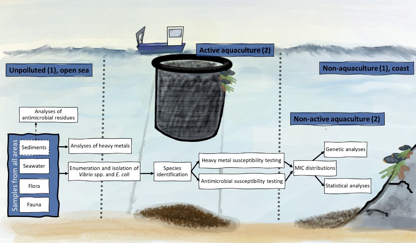
Et «Én-Helse»-perspektiv er viktig for å bedre forstå hvordan det marine miljøet påvirker seleksjon og spredning av antibiotikaresistens. Norsk akvakultur brukte store mengder antibiotika gjennom 80- og 90-tallet, og antibiotikaresistens blant fiskepatogene bakterier ble den gang sett i utstrakt grad. I tillegg har akvakulturnæringen siden sin oppstart brukt kobber som antibegroingsmidler i merdnøter og som tilskudd i fiskefôr. Som et resultat av dette har noen akvakulturanlegg høye konsentrasjoner av kobber i sedimentene under merdene. Flere studier har rapportert at tungmetall, også i lave konsentrasjoner som ikke hemmer bakterier, kan selektere for både tungmetall- og antibiotikaresistens. I dette studiet ble Vibrio spp. benyttet som en marin indikatorbakterie for antibiotika- og tungmetallresistens i kobberforurensende områder. Seks ulike lokasjoner ble prøvetatt ved to separate tidspunkt. Områdene ble delt inn i fire kategorier etter påvirkning fra akvakultur: Aktiv akvakultur, Ikke-aktiv akvakultur, Ikke-akvakultur og Rene områder. Totalt 70 prøver, inkludert sedimenter, sjøvann, marin fauna og marine alger, ble undersøkt for forekomst av Vibrio spp. og indikatorbakterier for fekal forurensing (Escherichia coli). Sedimentene ble også undersøkt for tungmetaller, hvor akutt toksiske konsentrasjoner ble funnet ved de Aktive akvakulturområdene med et gjennomsnitt på 272,3 mg/kg tørrvekt (t.v.) for kobber, signifikant høyere sammenlignet med Ikke-aktive (24,4 mg/kg t.v.), Ikke-akvakultur (34,8 mg/kg t.v.) og Rene områder (2,28 mg/kg t.v.), samt moderat toksiske konsentrasjoner med et gjennomsnitt på 474,6 mg/kg t.v. for sink, også signifikant høyere sammenlignet med Ikke-aktiv (70,7 mg/kg t.v.), Ikke-akvakultur (144,6 mg/kg t.v.) og Rene områder (16,4 mg/kg t.v.). Blant de 350 undersøkte Vibrio splendidus isolatene og de 72 Vibrio anguillarum isolatene, var størsteparten følsomme for alle de antibiotika de ble testet mot. Høyere minste hemmende konsentrasjon ble sett for oksytetrasyklin og kobber blant noen isolater fra Aktive akvakulturområder, men dette var kun én-til-to ganger høyere enn blant isolater fra Ikke-aktiv akvakultur og Ikke-akvakulturområdene. Flere antibiotika- og tungmetallresistensgener ble funnet i alle de undersøkte områdene, med unntak av genet nlpE, som kun ble funnet ved et akvakulturområde. Dette genet koder for et kobbersensorprotein som induserer membranpumper som skiller ut ulike uønskede substanser. Størsteparten av de 336 undersøkte E. coli isolatene var følsomme for alle antibiotika de ble testet mot. De Aktive akvakulturområdene hadde høyeste antall E. coli, og også flest av de resistente E. coli isolatene. Det er likevel mange faktorer som påvirker tilførselen av E. coli fra kloakk og avrenning fra land, slik som værforhold og topografien til området. Det ble ikke funnet noe sammenheng mellom resistens hos V. splendidus og E. coli ved noen av de undersøkte områdene, hvor flere prøver fra flere lokaliteter trolig vil kunne gitt bedre nyanser rundt de observerte forskjellene. Basert på den høye forekomsten av sensitive bakterieisolater, konkluderes det med at det er lav forekomst av resistensmekanismer blant vibrioer som det kan som det kan selekteres for i de undersøkte kobberforurensede områdene.
Screening for antimicrobial- and heavy metal resistant bacteria in copper contaminated areas
Report series:
Rapport fra havforskningen 2021-18
ISSN: 1893-4536
Published: 22.04.2021
Project No.: 15319
On request by: Miljødirektoratet
Reference: M-1925|2021 Kontraktsnr: 18087148
Research group(s):
Fremmed- og smittestoff (FRES)
Subject:
Mikroorganismar i havet og i sjømat
Program:
Trygg og sunn sjømat
Approved by:
Research Director(s):
Gro-Ingunn Hemre
Program leader(s):
Livar Frøyland
Norsk sammendrag
Summary
A One heath approach is essential to examine the role of the marine environment in the selection and spread of antimicrobial resistance. Norwegian aquaculture used high amounts of antimicrobials during the 80s and 90s, which facilitated widespread resistance among fish pathogens. Moreover, fish farms have since their beginning used copper containing coating as anti-fouling agents on the fish nets, in addition to copper supplements in the fish feed. Consequently, some fish farms have high concentrations of copper in det sediments beneath the pens. Several studies have reported that even sublethal concentrations of heavy metals can facilitate co-selection of antimicrobial resistance and heavy metal resistance. This study applied Vibrio spp. as indicator of antimicrobial- and heavy metal resistance in copper contaminated areas. Six different locations were sampled twice. These represented four different areas in regard of aquaculture activity; Active aquaculture, Non-active aquaculture, Non-aquaculture and Unpolluted. In total, 70 samples, including sediments, seawater, marine fauna and marine algae, were examined for the presence of Vibrio spp. and Escherichia coli. The sediments were examined for heavy metals, where sediments from Active aquaculture areas held exstensively toxic mean concentration with 272.3 mg/kg dry weight (d.w.) copper, significant higher than Non active (24.4 mg/kg d.w.), Non-aquaculture (34.8 mg/kg d.w.) and Unpolluted (2.28 mg/kg d.w.), and moderate toxic mean concentration with 424.6 mg/kg d.w. zinc, also significant higher than Non-active (70.7 mg/kg d.w.), Non-aquaculture (144.6 mg/kg d.w.) and Unpolluted (16.4 mg/kg d.w.). The majority of the retrieved 350 Vibrio splendidus and 72 Vibrio anguillarum isolates were susceptible to all the antimicrobials tested for. Increased minimum inhibition concentrations (MIC) to oxytetracycline and copper were seen for some isolates from Active aquaculture, however only one- to two-fold higher than from Non-active and Non-aquaculture areas. Several antimicrobial- and heavy metal resistance genes were found across the different examined areas, with exception of the nlpE gene encoding a copper sensing lipoprotein inducing efflux pumps, that were only found in one isolate from one location with aquaculture. The majority of the 336 E. coli isolates were susceptible to all antimicrobial tested for. The Active aquaculture areas conferred highest number of E. coli, and most of the resistant E. coli. Many factors, such as weather and topography, can influence the inflow of E. coli from sewage and run-offs from land. No association was found between the detected phenotypic and genotypic resistance traits in V. splendidus and in E. coli in any of the examined areas. Importantly, a higher sample size including more locations is needed to determine whether any possible indicated differences are significant. In conclusion, the high proportion of susceptible isolates found in this project, indicates that the prevalence of selectable resistance mechanisms in the examined marine vibrios from copper contaminated areas are low.
1 - Abbreviation
| AMP | Ampicillin |
| AMR | Antimicrobial resistance |
| ARGs | Antimicrobial resistance genes |
| AST | Antimicrobial Sensitivity Testing |
| AZM | Azithromycin |
| CAZ | Ceftazidime |
| CIP | Ciprofloxacin |
| CHL | Chloramphenicol |
| CST | Colistin |
| CTX | Cefotaxime |
| d.w. | dry weight |
| ECV | Epidemiological cut-off value |
| FLO | Florfenicol |
| HMRGs | Heavy metal resistance genes |
| GEN | Gentamicin |
| MEM | Meropenem |
| NAL | Nalidixic acid |
| NIT | Nitrofurantoin |
| OTE | Oxytetracycline |
| OXA | Oxolinic acid |
| SMZ | Sulfamethoxazole |
| TET | Tetracycline |
| TGC | Tigecycline |
| TMP | Trimethoprim |
| w.w. | wet weight |
2 - Background
Norwegian fish farming in net pens impact the biotic and abiotic environment surrounding the facilities in multiple ways. In the 1980s and 90s, large quantities of antimicrobials were used to treat bacterial infections in fish and a significant increase in antimicrobial resistant bacteria in sediments near fish farms were detected [1]. The highest consumption was in 1987, with close to 50 tonnes measured as pure substance of antimicrobials, including 21 130 kg of oxytetracycline, 15 840 kg of nitrofurazolidone, 3 700 kg of oxolinic acid and 1 900 kg of trimethoprim/sulfadiazine (sales statistics from the Norwegian Medicinal Depot AS). Following the development of effective vaccines against vibriosis (Vibrio anguillarum), cold-water vibriosis (V. salmonicida) and furunculosis (Aeromonas salmonicida) in the 1990s [2, 3], there has been a sharp reduction in the use of antimicrobials in fish farming, and the five-year average 2015-2019 was 452 kg, comprising 321 kg florfenicol, 125 kg of oxolinic acid and 6 kg of oxytetracycline [4]. A significant proportion of these drugs were, however, for the treatment of farmed cleaner fish for salmon lice control, and not for the breeding of fish for human consumption [4, 5].
The use of antimicrobials is recognised as the strongest driver for antimicrobial resistance, but other substances also stimulate the selection of resistance in bacteria. This applies in particular to heavy metals, such as copper, zinc and cadmium [6, 7]. High concentrations of heavy metals are bactericidal, and exposed bacteria therefore develop resistance for protection. Among the heavy metals discharged into the sea from various sources in Norway, it is estimated that copper input is the greatest with 1 251 tonnes in 2016, followed by zinc with 576 tonnes [8]. Unlike many types of antimicrobials, metals do not break down and will therefore accumulate and probably have long lasting effects on the surrounding environment. Today's aquaculture activity does not use and discharge significant quantities of antimicrobials into the sea, but fish farming is still considered as the greatest contributor of copper due to the use of copper containing anti-fouling agents on fish nets, and direct discharge of copper-enriched fish feed. The risk report for fish farming from 2018, showed that sediments in some areas were classified as toxic (Table A1) e.g., above 84 mg/kg dry weight (d.w.) [9]. Furthermore, sublethal concentrations of antimicrobials [10] and heavy metals [11] have been shown to select for antimicrobial resistance.
The mechanisms of heavy metal resistance may be the ability to reduce the toxicity by binding and forming complexes, or by reducing the metal ions to less toxic forms. A third mechanism is excretion through membrane pump systems [6, 12]. The presence of such complex pumping systems in some bacteria can result in co-resistance to a variety of antimicrobials, and several links between heavy metal resistance and antimicrobial resistance have been found. However, it is the co-localization of heavy metal resistance genes (HMRGs) and antimicrobial resistance genes (ARGs) on mobile genetic elements, such as transposons and plasmids that allow selection of both genes, when exposed to one of the selective factors. For instance, when pigs were fed copper supplemented feed, the copper resistance gene tcrB and the gene encoding resistance to erythromycin ermB were simultaneously selected for in Enterococcus faecalis and E. faecium [13]. Such co-selection of resistance mechanisms could also happen in the environment and promote the spread of resistance genes within or between bacterial species. It is plausible to hypothesise that continuous discharge and exposure of heavy metals may sustain the selection pressure for some antimicrobials even though the drug is no longer discharged [14].
Antimicrobial resistant bacteria in the marine environment are a major collective term for all bacteria in the ocean that are able to grow at antimicrobial concentrations above the wild type levels. These bacteria represent large parts of the marine microbiota and cannot be easily described or classified. They include bacteria in water and sediments, on seaweed and kelp, and in and on larger organisms, such as bivalves, crustaceans and fish. Some bacteria are restricted to one of these habitats, while others may be ubiquitous [15]. In addition, some non-marine bacteria such as Escherichia coli that are predominantly from homeothermic animals, including humans, may contaminate aquatic environments for instance through run-offs from agricultural areas or sewage facilities. Mobile resistance mechanisms that are of special concern in a One Health perspective may then be of importance, like extended spectrum beta-lactamases and plasmid mediated quinolones resistance. Several marine bacteria harbour intrinsic resistance properties to several antimicrobials, which are unlikely to be shared and thus not spread between species. Nevertheless, many marine bacteria are particularly prone to pick up foreign genes and collect different resistance properties. Some of these bacteria are also opportunistic pathogens, and since they often have a high degree of intrinsic resistance, there is a limited choice of antimicrobial for treatment. It is therefore important to investigate both intrinsic and acquired resistance in marine bacteria. There are currently no established or validated marine indicator organism for antimicrobial resistance in the same way as it is for antimicrobial resistance surveillance in production animals and meat (e.g., E. coli and Enterococcus spp.).
Vibrio is a true marine genus containing about 140 species, where 12 species are known to be pathogenic to humans and several more pathogenic to marine animals, such as fish and oysters. The ability of vibrios to tolerate elevated levels of copper depends on their habitation and environmental conditions. Shi et al. found that the vibrio-host oysters, accumulate copper for antibacterial effect [16], and Vanhove et al. found that copper resistance genes cusCBAF and copA gave beneficial virulent traits in vibrios and were necessary for surviving intracellularly when infecting the host [17]. Different Vibrio species have intrinsic resistant features developed by evolution, and not by recent acquired genes, such as the tetracycline resistance gene tet(34), the chloramphenicol resistance genes catB and bcr/cflA, and the multidrug efflux pump gene emrD [18, 19], however, these resistance traits are not necessarily expressed phenotypically if not needed [20]. Furthermore, resistance to ampicillin and colistin in V. anguillarum have been found to be related to whether it is serovar O1 or O2 [21]. Both the human pathogenic and non-pathogenic Vibrio species are also competent to acquire antimicrobial resistance genes. For instance, other tet genes coding for efflux pumps, conferring resistance to tetracyclines, have been found in V. splendidus and V. tasmaniensis [22], and on an R plasmid in V. anguillarum [23]. Other genes, such as blaNDM-1[24], blaCTX-M and qnrA [25, 26] encoding beta-lactam and quinolone resistance, respectively, have also been found in human pathogenic vibrios. Some vibrios also harbour the metallo-beta-lactamase varG gene, which has its strongest activity against meropenem [27].
Antimicrobial resistance associated with the aquaculture industry is a recurring topic. Since it has been shown that heavy metals can induce and sustain antimicrobial resistance, there is a need to identify whether bacteria have acquired resistance to antimicrobials used in the 1980s and 1990s, as well as if the bacteria present at aquaculture locations are impacted by the continuous discharge of heavy metals into their environment. Hence, the aim of this project was to screen for antimicrobial and heavy metal resistance among marine Vibrio species and the faecal indicator organism E. coli.
3 - Materials and methods
3.1 - Locations
To investigate the presence of antimicrobial and heavy metal resistant bacteria in the marine environment and the possible relationship to copper discharges, samples were collected from two active aquaculture sites, referred to as Active aquaculture areas. These sites had known use of fish nets with anti-fouling agents and historical high concentrations of copper in sediments (information obtained from Fylkesmannen in Hordaland). Two closed aquaculture locations that were investigated for antimicrobial resistance in the early 90's were included to see if the resistance pattern changes after the production stops, referred to as Non-active aquaculture areas. Further two areas were included, both far away from aquaculture, one located close to shore (Non-aquaculture) and one in the open sea (Unpolluted).
3.2 - Sampling
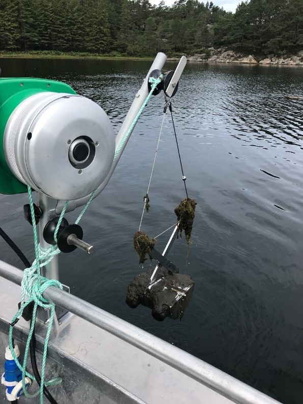
Each location was sampled twice and from each sampling we aimed for six samples consisting of two samples of sediments, two water samples, one fauna sample (molluscs), and one flora sample (macroalgae). The sediments at the aquaculture locations were sampled with a large Van Veen Grab used for recipient analyses. At other locations, a small Van Veen Grab was used (Figure 2). Molluscs and macroalgae samples were collected in sterile plastic bags using sterile glows and sometimes tweezers and knives, into sterile plastic bags. The water samples were collected by a clean 3 litre Van Dorn water sampler and transferred to acid washed Teflon bottles. The fauna and flora samples were collected in sterile plastic bags using sterile gloves and tweezers. All samples were kept cold during transport, and microbial analyses started within 24 hours.
3.3 - Chemical analyses
3.3.1 - Analyses of heavy metals
The concentration of heavy metals in samples of sediments, fauna and flora were analysed in inductive-coupled plasma mass spectrometer (ICPMS) by a standardised accredited protocol for sample preparation and heavy metal detection [28]. All samples were freeze-dried prior to analyses, and the sediment samples were additionally sieved through a 500µm mesh, and the smaller fraction was analysed. The seawater samples were examined by inductive-coupled plasma sector field mass spectrometer (ICP-SFMS) according to SS EN ISO 17924-1,2 and inductive-coupled plasma atomic emission (ICP-AES) according to ISO 11885, and the analyses were performed by ALS Laboratory Group Norway. The data sets were analysed for outliers, and one-way Anova (GraphPad Prism v8) was used for statistical comparison between areas.
3.3.2 - Screening for antimicrobial residues
The samples were examined by Liquid chromatography–mass spectrometry/mass spectrometry (LC-MS/MS) screening for multiple antimicrobials. It is expected that antimicrobials will have longer half-life in sediments compared to water, fauna and flora samples. Sediment samples from all locations were therefore examined for residues of the antimicrobial's ciprofloxacin, enrofloxacin, oxolinic acid, flumequine, trimethoprim, and florfenicol. Additionally, four samples from Active aquaculture areas and two samples from Unpolluted areas, were also analysed for tetracycline, oxytetracycline, doxycycline and chlortetracycline.
3.4 - Quantitative and qualitative isolation
3.4.1 - Isolation of Vibrio spp.
1) Each sample of sediment, fauna and flora was quantitatively examined for Vibrios using one or both of the following selective methods: a) 10-fold dilutions with peptone water and spread on VibrioChromo-select agar and incubated at 25 °C for 48 hours. The limit of quantification (LOQ) was 10 colony forming units (CFU)/g. b) Most probable number (MPN) for Vibrios with 3x5 tubes dilution series with alkaline peptone water [29] for 48 hours and confirmation on VibrioChromo-select agar grown at 25 °C for 48 hours. The LOQ was 18 bacteria/100g.
2) Seawater samples were filtered through a 0.45µm filter in aliquots of 2x 100 ml and 2x 50 ml per filter and grown on VibrioChromo-select agar at 25 °C for 48 hours. LOQ was 1 CFU/50 ml.
3) From each sample, up to 20 different colonies were grown to pure culture and identified by matrix-assisted laser desorption/ionization time-of-flight mass spectrometer (MALDI-TOF MS, MALDI Biotyper®, Bruker) at the Norwegian Veterinary Institute (NVI), Bergen, using a combination of the reference library from Bruker and an «in-house» library created by the NVI. The bacteria were frozen in 25% glycerol and stored at -80 °C.
3.4.2 - Isolation of Escherichia coli
1) Each sediment sample, fauna sample and flora sample were analysed a) Quantitatively for E. coli using standardized MPN methodology [30] confirmed on TBX agar. The LOQ was 18 CFU/100g. b) Qualitatively for Enterobacteriaceae on MacConkey agar grown at 37 °C for 24 hours. Typical pink colonies were verified on Chromagar before making pure cultures. LOQ was 10 CFU/g.
2) Water samples were filtered in aliquots of 1x 200 ml and 1x 500 ml per filter and grown on MacConkey agar at 37 °C for 24 hours. The LOQ was 1 CFU/200 ml.
3) Up to 20 E. coli isolates from each sample were grown to pure culture and identified by MALDI-TOF MS at the NVI, Oslo, before frozen in 25% glycerol and stored at -80 °C.
3.5 - Phenotypic susceptibility testing
The bacterial isolates were tested for susceptibility to 1) at least eight antimicrobials and 2) the heavy metals copper, zinc and cadmium.
3.5.1 - Heavy metal susceptibility testing
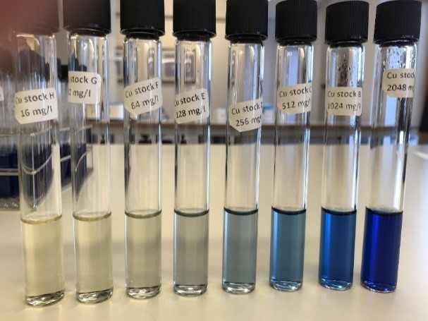
Investigation of heavy metal resistance was carried out in 96-well plates with increasing concentration of copper, zinc or cadmium. For each heavy metal, a stock solution was prepared and used to make two-fold dilutions to obtain the range from 2 048 mg/L to 16 mg/L for copper (Figure 3) and zinc, and 1 024 mg/L to 8 mg/L for cadmium. The metals were dissolved in 50 ml dH2O and subsequently added 50 ml double strength Mueller Hinton broth. For Vibrio splendidus, the Mueller Hinton broth contained 4% NaCl. Overnight cultures were dissolved in sterile water with or without 2% NaCl to obtain 0.5 MacFarland and 30 µl were transferred to tubes with 5 ml Mueller Hinton broth with or without 2% NaCl. The plates were filled by using AIMs dispenser by first dispensing the different concentrations of the heavy metals followed by dispensing the sample. The plates were covered with plastic film for 24-48 hours. The first well without growth were recorded as minimum inhibition concentration (MIC) [31, 32].
3.5.2 - Antimicrobial susceptibility testing
Susceptibility to antimicrobials were tested using standard broth microdilution methods. For susceptibility testing of E. coli isolates, the Sensititre® EUVSEC panel (TREK Diagnostics, LTD.) was used. This panel contains the following substances, ampicillin, cefotaxime, ceftazidime, meropenem, tetracycline, tigecycline, sulfamethoxazole, trimethoprim, nalidixic acid, ciprofloxacin, gentamicin, chloramphenicol, colistin and azithromycin. Epidemiological cut-off values recommended by the European Committee on Antimicrobial Susceptibility Testing (EUCAST, accessed 23.03.2020) were used, except for azithromycin for which cut-off values are not defined. See Table A2. for definitions of cut-off values.
There are no similar standardized panel for Vibrio spp., and custom-made panels from Sensititre® (TREK Diagnostics, LTD.) were made. These plates contain ampicillin, cefotaxime, ceftazidime, meropenem, oxytetracycline, tigecycline, sulfamethoxazole, trimethoprim, oxolinic acid, ciprofloxacin, gentamicin, florfenicol, colistin, azithromycin and nitrofurantoin. Prior to analysis, different Vibrio spp. were tested for cultivation on Mueller Hinton media with or without 2% NaCl. For V. splendidus, the addition of salt was needed to obtain growth. Plates were incubated at 25 °C for 24-48 hours. Since there are still no breakpoint values for Vibrio spp., an ECV was calculated for the combination of each of the Vibrio spp./antibiotics by ECOFFinder [33] based on the obtained MIC distribution data. ECV at 97.5% were applied, see Table A2. for definitions of cut-off values. Isolates with MIC above ECV are referred to as resistant, even though there is an uncertainty in the defined break-point as it is based on the data obtained in this project only.
3.6 - Data processing
Data from antimicrobial sensitivity testing (AST) were presented with 95% confidence intervals calculated by the exact binomial test using R version 3.5.2 for Windows (R Development Core Team, 2019). For Vibrio spp., the MIC distributions were analysed for differences in respect of sampling area for the tested antimicrobials and heavy metals by nonparametric OneWay Anova with KruskWallis test in GraphPad Prism 8.4.3 (©1992-2020 GraphPad Software, LLC). Susceptibility data for E. coli were recorded and stored as discrete values (MIC). Data management and analysis were performed in SAS-PC System® v 9.4 for Windows (SAS Institute Inc., Cary, NC, USA) and in R v4.03 [34].
Graphs were made in GraphPad Prism 8.4.3 (©1992-2020 GraphPad Software, LLC) and Microsoft® Excel® for Microsoft Office 365® ProPlus. Pearson correlation test was performed to tests for possible pairwise correlations between the occurrence of specific resistances towards antimicrobials and the heavy metals copper, zinc and cadmium in samples where both Vibrio spp. and E. coli had been isolated (N=147).
3.7 - Genotypic resistances testing
Bacterial isolates with special resistance patterns were subjected to whole-genome sequencing. DNA from the Vibrio isolates were extracted with Qiagen Blood and Tissue kit (Qiagen). Library preparations were performed applying Swift Turbo 2S flex prior to sequencing with Illumina MiSeq with 2 x 300 bp, both steps performed at the Norwegian Sequencing Centre (Oslo). Paired end reads were trimmed in bbMAP 31 [35] and assembled applying SPAdes v.3.13.0 [36]. Genomes were blasted against BacMet predicted database v2.0 [37] to assess heavy metal resistance genes. The genomes were also uploaded to National Center for Biotechnology Information, where the genomes were annotated prior to manual assessment of resistance genes.
DNA from the E. coli isolates were extracted using Qiagen QIAamp® Mini kit (Qiagen). The DNA extracts were sequenced at the NVI using Illumina® MiSeq with Nextera DNA Flex library prep. Paired end reads were trimmed and assembled using the Bifrost pipeline [38]. Assemblies were subjected for analysis for both acquired genes and chromosomal point mutations using the ResFinder v4.1 pipeline at the Centre for Genomic Epidemiology web site (https://cge.cbs.dtu. dk/services/ResFinder/) [39, 40].
3.8 - Microbiome
From each sediment sample, microbiome analyses were prepared for 16S rRNA gene amplicon sequencing, to compare the overall microbial (bacterial and archaeal) richness and diversity between locations. Sequence data was processed using the DADA2 [41] software implemented in the Qiime2 [42] pipeline, to construct ASVs (Absolute Sequence Variants), where each ASV represents one bacterial or archaeal species. Statistical analyses to compare sample diversity between locations was done using R (R core team, 2020, https://www.R-project.org) calculating Shannon index for each sample. This index is a function of number of species observed, and the evenness of their distribution within a community. A high Shannon diversity is usually considered to be a sign of a healthy environment, whereas low Shannon diversity can be a sign of the opposite.
4 - Results
4.1 - Sampling
Successful sampling was carried out twice at six different locations representing four different areas. Table 1 shows sampling position, description of the site, obtained samples and date of sampling. We failed to get a complete sample set at two locations and this was compromised by increasing the number of samples that were accessible. In total, 70 samples were collected.Table 1. Information about locations, sampling dates and samples taken twice at four different areas.
Table 1. Information about locations, sampling dates and samples taken twice at four different areas.
| Area | Location | Positions | Description | Depth | Water temp. | Samples | Date Sampled |
|---|---|---|---|---|---|---|---|
| Active aquaculture | 1 | Anonymous | Active fish farming site licenced since 1973, with annual fish production of 2600 tonnes using on average 3300 tonnes fish feed. | 500‑600 m, steep rocky bottom with sludge sediment pockets. | 12 °C, 8 °C | Water(2+2) Sediment(1+2) Fauna(2+1) Flora(2+1) | 30.10.2018 26.03.2019 |
| 2 | Anonymous | Active fish farming site licenced sin 1973, located 20 km from Location 1. Average fish production is 1800 tonnes using approx. 2250 tonnes fish feed. | 100‑250 m, gravel and sludge sediment pockets. | 12 °C, 11 °C | Water(2+2) Sediments(2+2) Fauna(0+0) Flora(2+1) | 14.11.2018 07.10.2019 | |
| Non‑active aquaculture | 5 | N60° 07' E5°13' | Kobbavika, Austevoll. Aquaculture site closed in 2008. | 7‑15 m, shell sand | 5 °C, 17 °C | Water(2+2) Sediments(2+2) Fauna(1+1) Flora(1+1) | 05.03.2019 13.08.2019 |
| 6 | N60° 16' E5°05' | Skogsvågen, Sotra. Closed aquaculture site examined for antimicrobial resistant Vibrio salmonicida in 1988 [1]. | 4‑13 m, gravel | 5 °C, 15 °C | Water(2+2) Sediments(2+2) Fauna(1+1) Flora(1+1) | 05.03.2019 09.09.2019 | |
| Non‑aquaculture | 4 | N59° 55' E5°15' | Pilapollen, Fitjar, a semi‑closed, shallow bay protected from aquaculture impact, with small boat travellers during the summer months. | 6‑10 m, muddy bottom | 5 °C,18 °C | Water(2+2) Sediments(2+2) Fauna(1+1) Flora(1+1) | 17.02.2019 13.08.2019 |
| Unpolluted | 3 | N58°58' E02°11' and N58°21' E1°49' | North Sea (3A) and Norwegian Sea (3B) (Control location) | 70 m and ca.100 m, gravel | 10 °C, 10 °C | Water(2+2) Sediments(2+2) Fauna(0+2 fish) Flora(0+0) | 16.11.2018 30.05.2019 01.10.2019 |
4.2 - Sample description
4.2.1 - Water samples
Water samples were obtained from all locations and the aim was to have sampling points with different water temperatures. However, for three of the locations, the temperatures were quite similar. The sampling at these locations was carried out between 5 – 11 months apart. For Location 3 this is as expected as the temperature in the North Sea does not vary that much.
4.2.2 - Sediment samples
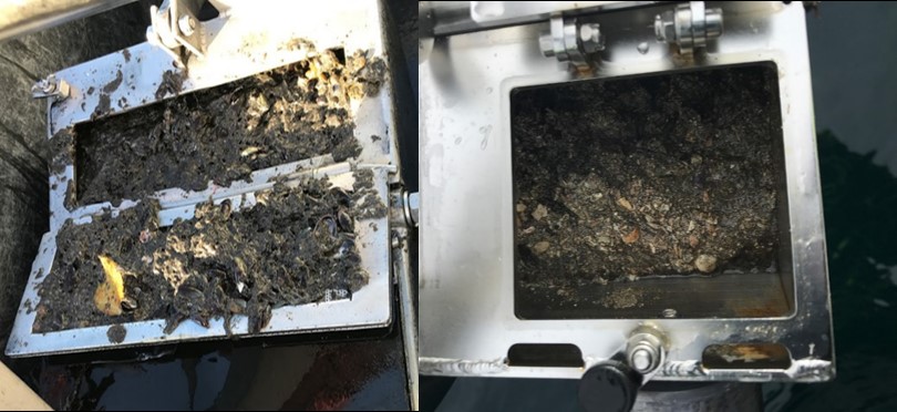
Sediment samples were also collected from all locations, with one sample missing at Location 1. This was caused by the uneven bottom topography at the location, where all grab hauls except one, came back empty. The bottom at this location is characterised as “rocky bottom”. Furthermore, the sediments from the different locations varied in composition where the Active aquaculture areas had sludge sediments, the Non-active aquaculture areas had shell sand and gravel, the Non-aquaculture area had mud sediments, and the Unpolluted areas contained gravel sediments. This means that the sediments also differed in grain size distribution (not measured) which impact the sediments ability to retain heavy metals and antimicrobials. Furthermore, the sludge sediments have high production of hydrogen sulphide (H2S) having anaerobic conditions (Figure 4) that could impact on the retrieved species.
The amount of organic material in the sediments were examined by subtracting the ash content (g/100g) from the dry matter content (g/100g), showing that the sludge samples from Active aquaculture had higher content of organic material (Figure 5).
4.2.3 - Marine fauna samples
The marine fauna samples comprised mostly of blue mussels (Mytilus edulis). At one Non-active aquaculture location, only limpets (Patella vulgata) could be found. They are grassing and not filtrating animals such as blue mussels but still represent quite stationary fauna from this location. Since there are no blue mussels growing in the North Sea, only fish were included as fauna. The fish samples were divided into fish skin/muscle and fish intestine.
4.2.4 - Marine flora samples
The flora samples comprised algae species that were accessible at the locations. For most areas this included brown algae such as bladder wrack (Fucus vesiculosus), sugar kelp (Saccharina latissima), channelled wrack (Pelvetia canaliculata) and rock weed (Ascophyllum nodosum). At one of the aquaculture locations, no brown algae were found, whereas scrapings of green algae (family Chlorophyta) were collected.
Further on, the samples are discussed according to area of origin.
4.3 - Microbiome in sediments
The effects of the aquaculture activity on the diversity and composition of the entire microbial community in the sediment samples was assessed using the 16S rRNA gene of bacteria and archaea.
A clear difference in microbial community structure was observed between sediment samples from Active aquaculture, Unpolluted and Non-active aquaculture areas (Figure 14). We also found higher overall Shannon diversity in samples obtained from Unpolluted and Non-active aquaculture areas than we did in the Active aquaculture areas (Figure 6), indicating a less healthy environment.
However, the sediment types also differed between the sampling areas (Figure 7). Sediment type and composition can be an important determinant of microbial community structure because of differences in nutrient and carbon availability. In addition, the sediments obtained from Active aquaculture areas had high H2S content, indicating they were most likely anaerobic. There are usually large differences in bacterial community compositions found in anaerobic sediments compared to aerobic sediments. It is therefore difficult to determine if the observed differences in this dataset is due to aquaculture activity or differences linked to sediment type (Figure A1).
4.4 - Heavy metals and antimicrobial residues in samples
All samples were examined for the heavy metals copper, zinc and cadmium by ICP-MS. One sample from a Active aquaculture area had the highest measured concentration of heavy metals with 2868.0 mg/kg d.w. copper and 774.4 mg/kg of zinc. Despite that this samples was considered an outlier, and were not inclueded in the mean concentrations, were sediment samples from Active aquaculture areas significantly higher than all other areas for both copper and zinc with mean of 272.3 mg/kg d.w. and 424.6 mg/kg d.w., respectively (Figure 8). This corresponds to extensively toxic (Class V) and moderate toxic (Class III) (Table A1), according to the classification of polluted environments [43]. Both the Non-active aquaculture and Unpolluted areas were classified with no toxic effect with mean concentrations of 9.8 mg/kg and 2.3 mg/kg, respectively, for the copper. The Non-aquaculture location had high levels of cadmium, which could be related to the mechanical industry with previous registered discharge of metals within 10 kilometres (Miljøstatus.no). Among the samples of blue mussels, the ones from Active aquaculture contained the highest concentration of copper (19.1 mg/kg d.w.), whereas for zinc and cadmium, the Non-aquaculture area were highest.
Analyses of heavy metals in seawater showed that the highest levels of copper and zinc were found at the Active aquaculture areas. None of the samples contained cadmium above the LOQ at 0.5 µg/l (Figure 9)
Among the sediment samples that were analysed for antimicrobial residues, none of the samples contained any antimicrobials above the LOQ of the applied method. List of examined samples, results and LOQ for the different antimicrobials are found in Table A3.
4.5 - Quantitative analyses and Culture collection
The prevalence of Vibrio spp. and E. coli were assessed quantitatively from all sample types. The results showed highest number of Vibrio spp. in flora and fauna sample at Active aquaculture areas (Figure A2), and highest number of E. coli in flora and fauna samples at the Non-aquaculture areas (Figure A3). However, in sediment samples and water samples analysed for E. coli, the highest concentrations were found in the Active aquaculture areas, 220 CFU/100ml and 31 CFU/100ml, respectively. The concentrations of E. coli indicate faecal pollution. In the water samples, the median value of E. coli was 7.1 CFU/100ml for Active aquaculture, 5 CFU/100ml for Non-active aquaculture, 6 CFU/100ml for Non-aquaculture and 0 CFU/100ml for Unpolluted. A clear difference was seen for samples sampled during October-March and April-September, where a 14-fold increase were seen in warmer months for Active aquaculture areas. For the Non-active aquaculture areas and the Non-aquaculture area, the increase were 5 and 6 folds higher during the warmer months.
From the same samples, 690 Vibrio isolates were obtained, and the two dominating species were selected for further analyses, and comprised 350 V. splendidus, 73 V. anguillarum. It was particularly challenging to sample Vibrio spp. from sediments with strong H2S-production.
Forty-three samples were presumptive positive for E. coli and 346 isolates were collected from these. Of these, 336 were confirmed to be E. coli. No E. coli were found from the samples originating from the Unpolluted areas at sea, which was expected.
Figure 11 shows the number of isolates from the different sample types.
4.6 - Phenotypic antimicrobial susceptibility testing
4.6.1 - Susceptibility according to areas
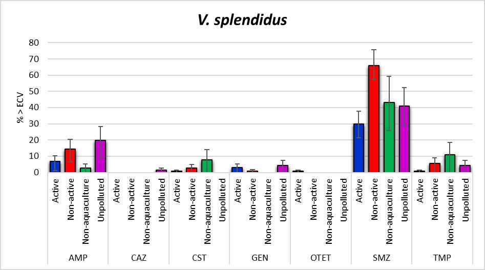
A total of the 759 isolates were tested for antimicrobial susceptibility. This included 350 V. splendidus, 73 V. anguillarum and 336 E. coli. An overview of the number of V. splendidus and E. coli isolates above ECV for the three species is shown in Figure 12. The isolates belonging to V. anguillarum showed only few isolates above ECV and the date are briefly presented in chapter 4.6.3 and in Table A4.
For V. splendidus 56.0% [95% CI: 50.6-61.3] were susceptible to all the antimicrobial classes tested for. The Active aquaculture areas had highest proportion of susceptible isolates with 71.0% [95% CI: 63.0-78.9], followed by Non-aquaculture areas with 57.0% [95% CI: 39.5-72.9], Unpolluted areas 56.3% [95% CI: 44.0-68.1] and Non-active aquaculture areas 37.0% [95% CI: 27.7-46.5].
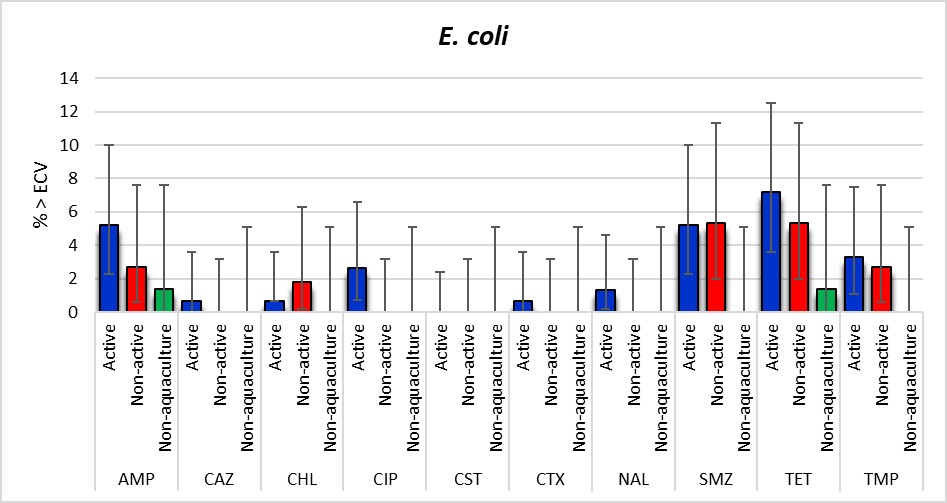
For E. coli, 91.7% [95% CI: 88.2-94.4] of the isolates were susceptible to all of the antimicrobial classes tested for, with a lower proportion in Active aquaculture areas and Non-active aquaculture areas with; 88.2% [95% CI: 82.0-92.9] and 92.0% [95% CI: 85.3-96.3], respectively, as compared to Non aquaculture areas with 98.6% [95% CI: 92.4-100.0].
4.6.2 - Vibrio splendidus
The antimicrobial susceptibility testing of 350 V. splendidus isolates (Figure 13) showed that growth above ECV were most common for sulfamethoxazole 44.9% [95% CI: 39.5-50.2], ampicillin [95% CI: 11.1 [8.0-14.9]] and trimethoprim 4.0% [95% CI: 2.2-6.6]. The Non-aquaculture areas had the highest proportion of isolates above ECV for ceftazidime, colistin, meropenem and trimethoprim. The Non-active aquaculture areas had the highest proportion of isolates above ECV for sulfamethoxazole, however, all the areas had high proportions above ECV for this agent. The Unpolluted areas had highest percentage above ECV for ampicillin. The Active aquaculture areas were the only areas that were above ECV for oxytetracycline and had four isolates showing one and two-fold higher MICs compared to all the other areas. However, a significant difference was seen for the MIC distribution of V. splendidus isolated from the Unpolluted areas compared to all the other areas, and not only for the Active aquaculture areas. None of the isolates were above the calculated ECV for azithromycin, cefotaxime, ciprofloxacin, florfenicol, nitrofurantoin, oxolinic acid and tigecycline. MIC distributions are presented in Table A5.
4.6.3 - Vibrio anguillarum
Antimicrobial susceptibility testing of 73 isolates belonging to V. anguillarum (Table A4) showed that MIC values were below the calculated ECV for 14 of the 15 agents included in the test panel. Seven isolates had MIC values above the ECV for colistin of 4 mg/L, and three of these were found in the Unpolluted areas. However, only four isolates were from these areas, thus the results are inconclusive.
4.6.4 - Escherichia coli
The most common resistances observed among the 336 E. coli isolates were to tetracyclines (5.4%; [95% CI: 3.2-8.3]), sulfonamides (4.2%; [95% CI: 2.3-6.9]) and ampicillin (3.6%; [95% CI: 1.9-6.2]) (Table A6). The proportion of resistance in the Active aquaculture and Non-active aquaculture areas was quite similar whereas only 1.4% of the isolates were resistant to ampicillin and tetracycline in the Non-aquaculture area. Only one isolate, which originated from the Active aquaculture areas, was resistant to third generation cephalosporins. However, as shown in Figure 14, any significant differences between the locations could not be detected. This is probably mainly explained by the low number of isolates obtained in the Non-aquaculture area. Four isolates were resistant to quinolones, ciprofloxacin and/or nalidixic acid. There were no isolates with resistance to gentamicin, meropenem or tigecycline observed.
4.7 - Heavy metal susceptibility testing
4.7.1 - V. splendidus and V. anguillarum
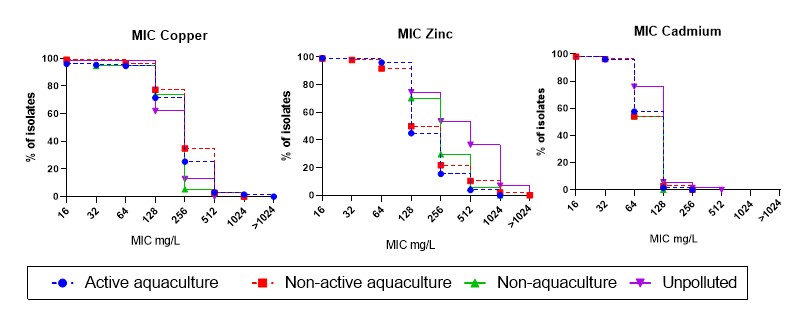
Both the V. anguillarum (Table A7) and V. splendidus (Table A8) were tested for susceptibility to the heavy metals copper, zinc and cadmium. Two V. splendidus isolates from Active aquaculture areas showed MIC above ECV for copper at >1024 mg/kg, and were two-fold higher than the isolates from the Unpolluted areas (Figure 15). However, only the Non-active aquaculture area showed significant higher MIC distribution for copper, compared to the Unpolluted areas, and only a trend was seen for the Active aquaculture areas. Resistance to zinc were seen in all areas with highest percentage of isolates from Unpolluted areas, followed by the Non-aquaculture area.
4.7.2 - E. coli
All E. coli isolates were tested for heavy metal susceptibility with the same concentrations as for the vibrios. Because of low variability of the results, no ECVs were calculated. Among the 336 isolates that were tested, 98% and 99% showed MIC above 1024 mg/L for copper and zinc, respectively. For cadmium, 95% had MIC of 128 mg/L, whereas 1.5% had MIC of 256 mg/L.
4.8 - Whole genome analyses
Whole genome sequencing was performed on a total of eleven V. splendidus, two V. anguillarum and four E. coli. All the Vibrio genomes harboured the tetracycline resistance gene tet(34), the chloramphenicol resistance gene catB and the multidrug efflux pumps encoded by the emrD gene and the bcr/cflA gene, the cadmium resistance gene cadA and the arsenite resistance gene acr3, all which are found in the reference genome of V. splendidus and V. anguillarum. Furthermore, some of the isolates harboured the trimethoprim resistance gene dfrA, beta-lactamase genes bla and ampC, and the quinolone resistance gene qnrS, in combination or alone (Table 2).
Searching for HMRGs revealed that all V. splendidus harboured several multidrug efflux systems such as RND (vmeD, vmeF, vmeI, vmeV, vmeY, vmeZ) and norM (vcmA), whereas some of the isolates carried additional multidrug efflux system genes, such as mtrF and vcrM (Table 5). The two V. anguillarum isolates carried the multidrug MFS transporter vceB. The arsenate resistance genes acr3 and aioB/aoxA were present in both V. splendidus and V. anguillarum isolates. One of the isolates from Active aquaculture areas harboured the nlpE gene encoding a copper sensing lipoprotein that induces stress response and activates efflux pumps. None of the known plasmid borne HMRGs such as zneB (zinc), czcC (cadmium, zinc), pcoA, copA, copB, copJ, cusB, (copper) [44], were detected.
| Areas | Isolate No. | Species | >ECV AB | ARGs | HMRGs | ||||||||
| dfrA | bla | ampC | qnrS | mtrF | vcrM | aioB/aoxA | vmeY | nlpE | vceB | ||||
| Active aquaculture | 2019‑397‑21 | V. splendidus | STX, TRIM | X | X | X | X | ||||||
| Active aquaculture | 2019‑399‑11 | V. splendidus | CST | X | X | X | X | ||||||
| Active aquaculture | 2018‑2091‑12 | V. splendidus | OTET | X | X | X | X | X | |||||
| Non‑active aquaculture | 2019‑184‑12 | V. anguillarum | X | X | |||||||||
| Non‑active aquaculture | 2019‑184‑17 | V. anguillarum | STX | X | X | ||||||||
| Non‑active aquaculture | 2019‑188‑18 | V. splendidus | STX, TRIM | X | |||||||||
| Non‑active aquaculture | 2019‑190‑8 | V. splendidus | STX, TRIM | X | X | X | |||||||
| Non‑active aquaculture | 2019‑193‑10 | V. splendidus | CST | X | X | X | X | ||||||
| Non‑active aquaculture | 2019‑195‑7 | V. splendidus | CST | X | X | X | X | ||||||
| Non‑active aquaculture | 2019‑196‑14 | V. splendidus | STX, TRIM | X | X | ||||||||
| Non‑active aquaculture | 2019‑195‑20 | V. splendidus | STX, TRIM | X | X | X | X | X | |||||
| Non‑aquaculture | 2019‑955‑15 | V. splendidus | CST, STX | X | X | X | |||||||
| Unpolluted | 2019‑1572‑18 | V. splendidus | STX, TRIM | X | X | X | |||||||
CST=colistin, STX=sulfamethoxazole, TRIM=trimethoprim, OTET=oxytetracycline
Among the four E. coli isolates which were subjected to whole genome sequencing, three were sequenced due to elevated MIC values for ciprofloxacin and/or nalidixic acid, while the last isolate expressed resistance to extended spectrum cephalosporins as well as quinolones and tetracyclines. In the three quinolone-resistant E. coli isolates, the resistance was due to one or two mutations in the chromosomally located gyrA gene (p.S83L and p.D87N) in two isolates and due to a plasmid mediated gene qnrS1 in the last isolate (Table 3). The resistance to extended spectrum cephalosporins was due to the blaCTX-M-15 gene. This isolate also harboured the qnrS1 and tet(A) genes conferring resistance to ciprofloxacin and tetracyclines, respectively.
Several genes associated with heavy metal resistance were detected (Table A9), and most of the genes are also found in reference E. coli genomes, including cusA, zntA, and several efflux pumps (acrB, acrD, mdtA, marA) involved in copper and zinc efflux. Two isolates harboured the plasmid borne pcoA gene, which encodes oxidoreductase proteins that detoxifies copper in the periplasm [45].
| Areas | Isolate | >ECV AB | ARGs | HMRGs | |||||
| blaCTX ‑M ‑15 | qnrS1 | tet(A) | gyrA (p.S83L) | gyrA (p.D87N) | pcoA | pcoS | |||
| Active aquaculture | 2019‑399‑2 | CIP, NAL | X | ||||||
| Active aquaculture | 2019‑400‑1 | CIP, NAL | X | X | X | ||||
| Active aquaculture | 2019‑400‑9 | CIP | X | X | |||||
| Active aquaculture | 2019‑604‑8 | AMP, TET, NAL, CIP, FOT, TAZ | X | X | X | X | X | ||
CIP=ciprofloxacin, NAL=nalidixic acid, AMP=ampicillin, TET=tetracyclines, FOT=cefotaxime, TAZ=ceftazidime
4.9 - Methodological considerations
This project tried to identify different Vibrio spp. that could function as indicator for antimicrobial resistance in the marine environment. Such an indicator should comply with some key characteristic being; 1) present in the tested environment, 2) being able to grow under laboratory conditions, and 3) express antimicrobial resistance relevant for surveillance.
Vibrio spp. showed some limitations, as they were not present in the anaerobic sediments containing H2S. This made it difficult to compare sediments from the different examined areas. Therefore, for further assessment of antimicrobial resistance in sediments, an alternative target bacterium needs to be identified.
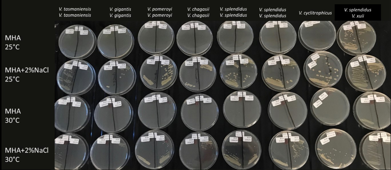
Furthermore, methods to perform AST in Vibrio spp. are not standardised in the same way as it is for surveillance of bacteria in food, veterinary and human medicine. AST testing of vibrios were therefore performed in custom-made 96-well Sensititre® plates (ThermoFisher) with protocol according to what is used in surveillance set up with adjustments of incubation temperature and time. The same adjustments were applied to isolates belonging to V. anguillarum or V. splendidus, whereas V. splendidus also needed additional salt added to the standardised Mueller Hinton growth media, and good growth was obtained by adding 2% NaCl to the broth. Furthermore, V. splendidus had poor growth after only 24 hours, hence incubation was extended to 48 hours to obtain good growth in the positive control well of the Sensititre® plates. The temperature was set at 25 °C which gave best growth for V. splendidus (Figure 16).
A complete sensitive strain of either V. splendidus or V. anguillarum was applied as control for both AST and heavy metal sensitivity testing. The controls were stable for all antimicrobial agents, and for zinc and cadmium. More variation was seen for copper. The use of Vibrio control strains needs more optimisation. As there is a need for low variability among similar analyses, having a fixed incubation time is crucial. A workaround for this could be to apply spectrophotometry to determine growth density and normalise the measured results according to the variations of the control strain.
The protocol for heavy metal susceptibility testing was performed in broth dilution according to Deus et al. [46], and differed only with the use of broth instead of agar as applied in previous work done on marine bacteria from Norway [32]. The major challenge when preparing growth media with high levels of heavy metals, such as for copper and zinc with 1024 mg/L, is the drop in pH, (pH 4 in copper solutions) when the metals are dissolved in water, and further their complex binding ability when pH increases too rapidly. This was solved by adjusting the solution with Na-Citrate, a weak base that slowly increased the pH to final pH 7. We applied the same concentrations for both Vibrio spp. and E. coli, but for E. coli this was not suitable. Higher metal concentrations should have been applied for this purpose.
5 - Discussion
This study aimed to examine antimicrobial and heavy metal resistance among Vibrio spp. and E. coli from locations with known heavy metal pollution. Active salmonid fish farms were chosen based on previous reported levels of copper in sediments below the net pens. In addition, two locations with previous aquaculture activity, one location without aquaculture activity, and one unpolluted location, were examined. Chemical analyses of the heavy metals copper, zinc and cadmium in sediments (Figure 8), confirmed significant elevated concentrations at the Active aquaculture areas, with a mean of 272.3 mg/kg d.w. copper and 474.6 mg/kg d.w. zinc, compared to the other tested areas. This corresponds to extensively toxic (Class V) levels of copper and moderate toxic (Class III) of zinc (Table A1). Sediments from Non-active aquaculture, Non-aquaculture and Unpollue areas held 24.4 mg/kg d.w., 34.8 mg/kg d.w., and 2.28 mg/kg d.w. copper, and 70.7 mg/kg d.w., 144.6 mg/kg d.w. and 16.4 mg/kg d.w. zinc, respsectively. Furthermore, the microbiome analyses (Figure 7) showing a decrease in microbial species diversity in the Active aquaculture areas, support that these areas are impacted by the fish farming activity.
Isolates belonging to V. anguillarum (n=73) and V. splendidus (n=350) were tested for antimicrobial susceptibility. The majority of V. anguillarum isolates were fully susceptible to all the antimicrobials tested for. Whereas, among the V. splendidus isolates, 56% were susceptible to all agents, 35.1%, 8.3% and 0.6% were above ECV for one, two and three or more antimicrobial classes, respectively. The overall high prevalence of susceptible isolates identified, reflects the low usage of antimicrobials in today’s fish farms and in Norway in general. During the 80s and 90s where high amounts of antimicrobials were used, both presence [1] and absence [47] of resistant bacteria was found beneath the net pens. The continued high use of antimicrobials can explain observed resistance in other aquaculture nations [48], such as Chile [49, 50] and China [51].
The Active aquaculture area had highest percentage of overall susceptible V. splendidus isolates. Active aquaculture areas were the only location that had one isolate with MICs above ECV for oxytetracycline (Figure 13). However, the isolates had overall MIC distribution similar to the MIC distribution of Non-active aquaculture and Non-aquaculture, and these three areas had all significant MIC distributions higher than the MIC distribution for isolates from the Unpolluted areas. The observed resistance to oxytetracycline could be related to tet(34) gene encoding a tetracycline inactivation enzyme that all vibrios harbour. The overexpression of tet(34) through regulatory response could have been induced from copper or zinc, as increased resistance to tetracycline have been seen after exposure to high [52] and even sublethal [11] concentrations of copper or zinc, rather than exposure of tetracycline itself. Håkonsholm et al. also found the tet(34) gene in all their Vibrio spp. that were isolated from open sea and herring, whereas none of the isolates expressed resistance after testing with disk diffusion [20]. One of the studies from aquaculture in the 90s found resistance to oxytetracycline in the majority of examined bacteria, and demonstrated that the tetracycline resistance mechanism from Vibrio spp. was transferable to E. coli [53]. Whether the increased resistance to oxytetracycline back then was linked to the historical use of oxytetracycline, exposure to heavy metals or both in combination, is not known, but this project did not identify any of such mobile tetracycline resistance genes.
Vibrio spp., including V. splendidus, have a unique ability to store multiple resistance genes that could easily be expressed whenever needed through cassettes in super integrons. This might explain the beta-lactamase genes, bla and ampC, and quinolone resistance gene qnrS, that were detected without the isolates showing any phenotypic resistance. Such silent resistance genes stored in cassettes are important for the robustness of the bacterium, being able to rapidly express genes necessary for survival in a changing environment. Hence, discharge of heavy metals to the marine environment can select for bacteria with such resistance genes, and also decrease bacterial diversity [54]. Further analyses including susceptible isolates will gain knowledge about unexpressed resistance genes.
The Active aquaculture areas were the only areas that had isolates above ECV for copper at >1024 mg/kg, however, the Non-active and Non-aquaculture areas had isolates with MIC at 1024 mg/kg, and no differences were seen between these area, and had were significantly higher MIC than what was found for the isolates from Unpolluted areas. Since we don’t know the true MIC for the isolates from Active aquaculture with MIC above the tested rage, these isolates should be examined more in detail.
Genes encoding multidrug efflux pumps and the arsenate efflux gene aioB/aoxA were found in isolates across the examined areas. One isolate from the Active aquaculture areas harboured an additional nlpE gene encoding copper sensing lipoprotein, which stimulates stress response and activates efflux pumps excreting both antimicrobials and heavy metals [55]. Unlike the other detected HMRGs, nlpE is associated to copper exposure, as it stimulates increased efflux of multiple drugs. This gene was recently detected in several Vibrio spp. genomes from open seawater in the North Sea [20], showing that this gene is not exclusive to Active aquaculture areas. Further examinations including whole genome sequencing and analyses of an extended number of isolates is needed to explore whether this or other HMRGs are more related to any of the areas included in the present survey.
The quantification of E. coli in all sample types showed that all areas, except for the Unpolluted areas where no E. coli was detected, were to some extent exposed to faecal pollution through sewage or run-offs from mainland. When comparing E. coli levels in seawater from all areas, a slightly increased, but not significant, inflow of faecal pollutions was implied at the Active aquaculture areas. These areas are located further inshore where less seawater is mixed, and thereby a lower dilution of faecal contamination is facilitated. The majority of the E. coli were fully susceptible to all antimicrobials tested for (91.7%). One of the E. coli showed resistance towards the extended spectrum cephalosporins, cefotaxime and ceftazidime, and the resistance was conferred by a blaCTX-M-15 gene. This isolate also harboured the qnrS1 gene conferring resistance to ciprofloxacin and tet(A) conferring resistance to tetracyclines. In one of three additional isolates expressing resistance to quinolones, the resistance was due to the plasmid mediated quinolone resistance gene qnrS1. E. coli with similar resistance pattern and genes as found in this study, have previously been found in marine bivalves in Norway [56]. The blaCTX-M-15 is part of the blaCTX-M resistance gene group 1, occasionally detected from humans and animals, both wild, domestic and livestock, in Norway [57-60]. The qnrS1 gene alone confers low level resistance to ciprofloxacin below the clinical cut offs set by EUCAST, but above the ECV. This gene has also occasionally been detected in samples from livestock and wild animals in Norway [60, 61]. Furthermore, two of the isolates harboured the plasmid borne pcoA gene encoding a copper efflux pump [62]. These four isolates were detected in water samples from the Active aquaculture areas. None of the E. coli isolated from the other areas showed any resistance to cephalosporins or quinolones. Furthermore, no correlation was seen between the phenotypic resistance results from V. splendidus and E. coli, indicating no link to faecal contamination. The E. coli results might among others be affected by weather conditions [63], such as precipitation that leads to increased run-off from land. Whether exposure to copper have affected the E. coli results could not be determined. More extensive studies on a higher number of Active aquaculture areas are needed to investigate these aspects further.
In conclusion, this project applied Vibrio spp. as indicators for antimicrobial- and heavy metal resistance in copper contaminated aquaculture areas compared to old aquaculture areas, a near shore non-aquaculture and a unpolluted off shore area. A possible association was seen in Active aquaculture areas where increased MIC values to oxytetracycline and copper were detected. Though slightly lower MIC values were seen for the Non-active and Non-aquaculture areas, no statistical differences could be found. Furthermore, antimicrobial resistance in V. splendidus did not correlate with the resistance found in E. coli. Importantly, selection for any resistance mechanism presupposes that the mechanism is present in the current environment. Given the high proportion of susceptible isolates found in this project, the overall prevalence of such selectable resistance mechanisms vibrios from copper contaminated areas assumed to be low.
This study has elucidated some challenges applied to the examination of antimicrobial resistant bacteria in copper contaminated aquaculture areas. We therefore suggest seven key points that should be considered in future surveys; 1) Identify indicator bacteria that are present in sediments containing high levels of H2S, 2) Increase number of locations to detect possible differences and changes, 3) Include multiple isolates from each location, 4) Establish species specific protocols for heavy metal susceptibility testing, 5) Perform genetic analyses of both susceptible and non-susceptible isolates, 6) Perform metagenomics on samples to investigate for both antimicrobial and heavy metal resistance genes, and 7) Combine future sampling with ongoing surveillance of aquaculture sites, such as Modelling-Ongrowing fish farms-Monitoring (MOM) or sampling associated with the “Risk assessment report of aquaculture”.
6 - Acknowledgement
We would like to thank the aquaculture company that welcomed our sampling and provided all the help we needed during sampling. We also thank Børge Alfstad, Heine Skaar Nilsen and Fredrik Håkonsholm for help with sampling, Betty Irgens for organisation of microbiological analyses, Hui-San Tung and Eva Myklebust for molecular analyses. Furthermore, a thank to Bente Solli, Nawarj Gautam, Snorri Gunnarsson, Rita Hannisdal and Tore Tjensvoll for chemical analyses, and Michael Bank and Atabak Mahjour Azad for help with method for testing heavy metals in water. Thanks to Bjørn Einar Grøsvik and Sepan Boitsov for important input on the sediement data. We would also like to thank Kingsley Oteng and Agathe Vikre Danielsen for performing the phenotypic analyses, and Kari Sandnes, Merete Gåsvær Sture and Kirsten Bottolfsen for performing the MALDI-TOF analysis.
7 - Appendicies
| Class I | Class II | Class III | Class IV | Class V | Reference | ||
|---|---|---|---|---|---|---|---|
| Sediments (mg/kg d.w.) | Copper | <20 | 84 | 84 | 147 | >147 | [43] |
| Zinc | <90 | 139 | 750 | 6690 | >6690 | ||
| Cadmium | <0.2 | 2.5 | 16 | 157 | >157 | ||
| Seawater (µg/L) | Copper | <0.3 | 2.6 | 2.6 | 5.2 | >5.2 | |
| Zinc | <1.5 | 3.4 | 6 | 60 | >60 | ||
| Cadmium | <0.03 | 0.2 | * | * | * | ||
| Brown algae (mg/kg w.w.) | Copper | <5 | 15 | 50 | 150 | >150 | [64] |
| Zinc | <150 | 400 | 1000 | 2500 | >2500 | ||
| Cadmium | <1.5 | 5 | 20 | 40 | >40 | ||
| Blue mussels (mg/kg w.w.) | Copper | <10 | 30 | 100 | 200 | >200 | |
| Zinc | <200 | 400 | 1000 | 2500 | >2500 | ||
| Cadmium | <2 | 5 | 20 | 40 | >40 |
| Antimicrobials | Escherichia coli | Vibrio splendidus | Vibrio anguillarum |
|---|---|---|---|
| Ampicillin | > 8 | > 4 | Intrinsic |
| Azithromycin* | ND | > 8 | > 8 |
| Cefotaxime | > 0.25 | > 0.5 | > 0.5 |
| Ceftazidime | > 0.5 | > 0.25 | > 4 |
| Chloramphenicol | > 16 | ND | ND |
| Ciprofloxacin | > 0.064 | > 0.5 | ND |
| Colistin | > 2 | > 1 | > 4 |
| Florfenicol | > 2 | > 1 | |
| Gentamicin | > 2 | >2 | > 4 |
| Meropenem | > 0.125 | > 0.25 | > 1 |
| Nalidixic acid | > 16 | ND | ND |
| Nitrofurantoin | ND | > 32 | > 0.12 |
| Oxolinic acid | ND | > 0.5 | > 0.12 |
| Oxytetracycline | ND | > 0.5 | > 0.5 |
| Sulfamethoxazole | > 64 | > 8 | > 8 |
| Tetracycline | > 8 | ND | ND |
| Tigecycline | > 0.5 | ND | ND |
| Trimethoprim | > 2 | > 4 | > 2 |
| Areas | DO* | CL-TET* | OXYTET* | TET* | ENRO | FLOR | FLUM | OXO | TRIM | CIP |
|---|---|---|---|---|---|---|---|---|---|---|
| Aquaculture | < 50 | < 50 | < 50 | < 50 | < 10 | < 4 | < 40 | < 40 | < 2 | NA |
| Aquaculture | < 50 | < 50 | < 50 | < 50 | < 10 | < 4 | < 40 | < 40 | < 2 | < 10 |
| Aquaculture | < 50 | < 50 | < 50 | < 50 | < 10 | < 4 | < 40 | NA | < 2 | < 10 |
| Unpolluted | < 50 | < 50 | < 50 | < 50 | < 10 | < 4 | < 40 | < 40 | < 2 | < 10 |
| Unpolluted | < 50 | < 50 | < 50 | < 50 | < 10 | < 4 | < 40 | < 40 | < 2 | < 10 |
| Non‑aquaculture | NA | NA | NA | NA | < 10 | < 4 | < 40 | < 40 | < 2 | < 10 |
| Non‑aquaculture | NA | NA | NA | NA | NA | < 4 | < 40 | < 40 | < 2 | NA |
| Non‑active aquaculture | NA | NA | NA | NA | < 10 | < 4 | < 40 | < 40 | < 2 | < 10 |
| Non‑active aquaculture | NA | NA | NA | NA | < 10 | < 4 | < 40 | < 40 | < 2 | < 10 |
| Non‑active aquaculture | NA | NA | NA | NA | NA | < 4 | < 40 | < 40 | < 2 | < 10 |
| Non‑active aquaculture | NA | NA | NA | NA | NA | < 4 | < 40 | < 40 | < 2 | < 10 |
| Aquaculture | NA | NA | NA | NA | < 10 | < 4 | < 40 | < 40 | < 2 | NA |
| Aquaculture | NA | NA | NA | NA | < 10 | < 4 | < 40 | < 40 | < 2 | < 10 |
| Aquaculture | NA | NA | NA | NA | NA | < 4 | < 40 | < 40 | < 2 | NA |
| Aquaculture | NA | NA | NA | NA | NA | < 4 | < 40 | < 40 | < 2 | NA |
| Non‑aquaculture | NA | NA | NA | NA | < 10 | < 4 | < 40 | < 40 | < 2 | < 10 |
| Non‑aquaculture | NA | NA | NA | NA | NA | < 4 | < 40 | < 40 | < 2 | NA |
| Non‑active aquaculture | NA | NA | NA | NA | < 10 | < 4 | < 40 | < 40 | < 2 | < 10 |
| Non‑active aquaculture | NA | NA | NA | NA | < 10 | < 4 | < 40 | < 40 | < 2 | < 10 |
| Non‑active aquaculture | NA | NA | NA | NA | NA | < 4 | < 40 | < 40 | < 2 | NA |
| Non‑active aquaculture | NA | NA | NA | NA | NA | < 4 | < 40 | < 40 | < 2 | NA |
| Unpolluted | NA | NA | NA | NA | NA | < 4 | < 40 | < 40 | < 2 | NA |
| Unpolluted | NA | NA | NA | NA | NA | < 4 | < 40 | < 40 | < 2 | NA |
Abbreviations: DO=doxycycline, CL-TET=Chlortetracycline, OXYTET=oxytetracycline, TET=Tetracycline, ENRO=Enrofloxacin, FLOR=Florfenicol, FLUM=Flumequine, OXO=Oxolinic acid, TRIM=Trimethoprim, CIP=Ciprofloxacin, NA=Not Analysed.
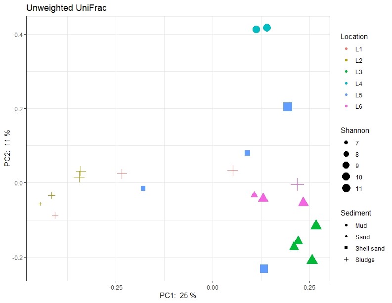 Figure A1. Principal component analysis illustrating similarity of samples regarding the activity of the sampling site and sediment type (shape of symbols) respectively. Shannon values (size of symbols) indicate the diversity of 16S sequences observed in the samples. The closer two points are on the plot, the more similar they are in microbial community composition. L1-L6 indicates locations as described in Table 1.
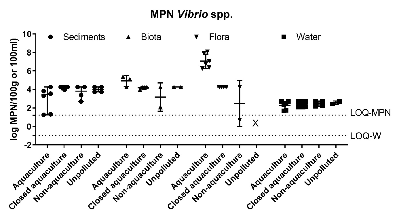
Figure A2. Quantitative analysis of Vibrio spp. in sediments, fauna, flora (mean ± range MPN/100g) and water (mean ± range CFU/100ml). The LOQ-MPN and the LOQ-W indicates the LOQ for the MPN method, and filtering method of water, respectively.
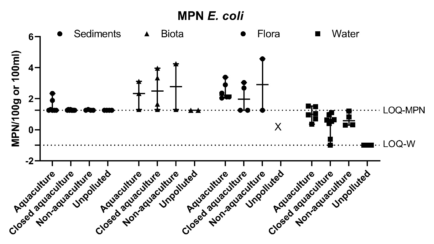
Figure A3. Quantitative analysis of E. coli in sediments, fauna, flora (mean ± range MPN/100g) and water (mean ± range CFU/100ml). The LOQ-MPN and the LOQ-W indicates the LOQ for the MPN method, and filtering method of water, respsectively.
| Number of isolates (n) of MIC values (mg/L) | ||||||||||||||
| % >ECV [95%CI] | 0.03 | 0.06 | 0.12 | 0.25 | 0.5 | 1 | 2 | 4 | 8 | 16 | 32 | 64 | ||
| AMP | Active aquaculture | Intrinsic | 27 | 3 | ||||||||||
| ECV:ND | Non‑active aquaculture | Intrinsic | 1 | 13 | ||||||||||
| Non‑aquaculture | Intrinsic | 7 | 18 | |||||||||||
| Unpolluted | Intrinsic | 4 | ||||||||||||
| Total | Intrinsic | 39 | 34 | |||||||||||
| AZM | Active aquaculture | 0.0 [0.0‑11.6] | 28 | 2 | ||||||||||
| ECV:>8 | Non‑active aquaculture | 0.0 [0.0‑23.2] | 14 | |||||||||||
| Non‑aquaculture | 0.0 (0.0‑13.7] | 25 | ||||||||||||
| Unpolluted | 0.0 [0.0‑60.2] | 4 | ||||||||||||
| Total | 0.0 [0.0‑4.9] | 71 | 2 | |||||||||||
| CTX | Active aquaculture | 0.0 [0.0‑11.6] | 27 | 3 | ||||||||||
| ECV:>0.5 | Non‑active aquaculture | 0.0 [0.0‑23.2] | 2 | 1 | 11 | |||||||||
| Non‑aquaculture | 0.0 (0.0‑13.7] | 14 | 6 | 5 | ||||||||||
| Unpolluted | 0.0 [0.0‑60.2] | 4 | ||||||||||||
| Total | 0.0 [0.0‑4.9] | 47 | 7 | 19 | ||||||||||
| CAZ | Active aquaculture | 0.0 [0.0‑11.6] | 2 | 26 | 1 | 1 | ||||||||
| ECV:>4 | Non‑active aquaculture | 0.0 [0.0‑23.2] | 2 | 12 | ||||||||||
| Non‑aquaculture | 0.0 (0.0‑13.7] | 14 | 11 | |||||||||||
| Unpolluted | 0.0 [0.0‑60.2] | 4 | ||||||||||||
| Total | 0.0 [0.0‑4.9] | 2 | 42 | 24 | 1 | |||||||||
| CIP | Active aquaculture | ND | 30 | |||||||||||
| ECV:ND | Non‑active aquaculture | ND | 14 | |||||||||||
| Non‑aquaculture | ND | 25 | ||||||||||||
| Unpolluted | ND | 4 | ||||||||||||
| Total | ND | 73 | ||||||||||||
| CST | Active aquaculture | 3.3 [0.1‑17.2] | 11 | 5 | 10 | 2 | 1 | 1 | ||||||
| ECV:>4 | Non‑active aquaculture | 7.1 [0.2‑33.9] | 8 | 5 | 1 | |||||||||
| Non‑aquaculture | 8.0 [1.0‑26.0] | 11 | 9 | 3 | 2 | |||||||||
| Unpolluted | 75 [19.4‑99.4] | 1 | 3 | |||||||||||
| Total | 9.6 [3.9‑18.8] | 11 | 5 | 29 | 17 | 4 | 7 | |||||||
| FLO | Active aquaculture | 0.0 [0.0‑11.6] | 28 | 2 | ||||||||||
| ECV:>1 | Non‑active aquaculture | 0.0 [0.0‑23.2] | 1 | 13 | ||||||||||
| Non‑aquaculture | 0.0 (0.0‑13.7] | 11 | 14 | |||||||||||
| Unpolluted | 0.0 [0.0‑60.2] | 4 | ||||||||||||
| Total | 0.0 [0.0‑4.9] | 39 | 32 | |||||||||||
| GEN | Active aquaculture | 0.0 [0.0‑11.6] | 2 | 19 | 8 | 1 | ||||||||
| ECV:>4 | Non‑active aquaculture | 0.0 [0.0‑23.2] | 3 | 10 | 1 | |||||||||
| Non‑aquaculture | 0.0 (0.0‑13.7] | 9 | 14 | 2 | ||||||||||
| Unpolluted | 0.0 [0.0‑60.2] | 3 | 1 | |||||||||||
| Total | 0.0 [0.0‑4.9] | 17 | 44 | 9 | 3 | |||||||||
| MEM | Active aquaculture | 0.0 [0.0‑11.6] | 9 | 21 | ||||||||||
| ECV:>1 | Non‑active aquaculture | 0.0 [0.0‑23.2] | 14 | |||||||||||
| Non‑aquaculture | 0.0 (0.0‑13.7] | 3 | 20 | 2 | ||||||||||
| Unpolluted | 0.0 [0.0‑60.2] | 4 | ||||||||||||
| Total | 0.0 [0.0‑4.9] | 12 | 59 | |||||||||||
| NIT | Active aquaculture | ND | 30 | |||||||||||
| ECV:ND | Non‑active aquaculture | ND | 14 | |||||||||||
| Non‑aquaculture | ND | 23 | ||||||||||||
| Unpolluted | ND | 4 | ||||||||||||
| Total | ND | 71 | ||||||||||||
| OXA | Active aquaculture | 0.0 [0.0‑11.6] | 30 | |||||||||||
| ECV:>0.12 | Non‑active aquaculture | 0.0 [0.0‑23.2] | 12 | 1 | 1 | |||||||||
| Non‑aquaculture | 0.0 (0.0‑13.7] | 24 | 1 | |||||||||||
| Unpolluted | 0.0 [0.0‑60.2] | 4 | ||||||||||||
| Total | 0.0 [0.0‑4.9] | 70 | 2 | 1 | ||||||||||
| OTE | Active aquaculture | 0.0 [0.0‑11.6] | 29 | 1 | ||||||||||
| ECV:>0.5 | Non‑active aquaculture | 0.0 [0.0‑23.2] | 14 | |||||||||||
| Non‑aquaculture | 0.0 (0.0‑13.7] | 4 | 21 | |||||||||||
| Unpolluted | 0.0 [0.0‑60.2] | 2 | 2 | |||||||||||
| Total | 0.0 [0.0‑4.9] | 35 | 37 | |||||||||||
| SMZ | Active aquaculture | 0.0 [0.0‑11.6] | 14 | 9 | 7 | |||||||||
| ECV:>8 | Non‑active aquaculture | 0.0 [0.0‑23.2] | 14 | |||||||||||
| Non‑aquaculture | 4.0 (0.0‑20.4] | 2 | 12 | 10 | 1 | |||||||||
| Unpolluted | 0.0 [0.0‑60.2] | 4 | ||||||||||||
| Total | 1.4 [0.0‑4.9] | 16 | 39 | 16 | 1 | |||||||||
| TGC | Active aquaculture | ND | 30 | |||||||||||
| ECV:ND | Non‑active aquaculture | ND | 14 | |||||||||||
| Non‑aquaculture | ND | 25 | ||||||||||||
| Unpolluted | ND | 4 | ||||||||||||
| Total | ND | 73 | ||||||||||||
| TMP | Active aquaculture | 0.0 [0.0‑11.6] | 5 | 13 | 12 | |||||||||
| ECV:>2 | Non‑active aquaculture | 0.0 [0.0‑23.2] | 2 | 10 | 2 | |||||||||
| Non‑aquaculture | 0.0 (0.0‑13.7] | 3 | 22 | |||||||||||
| Unpolluted | 0.0 [0.0‑60.2] | 4 | ||||||||||||
| Total | 0.0 [0.0‑4.9] | 5 | 18 | 48 | 2 | |||||||||
Aquaculture(n=30), Non-active aquaculture (n=14), Non-aquaculture (n=25) and Unpolluted (n=4). ECV=Epidemiological cut-off value. White fields indicate the tested range of antimicrobials concentrations. ND= not determined.
| Distribution (%) of MIC values (mg/L) | ||||||||||||||
| % >ECV [95%CI] | 0.03 | 0.06 | 0.12 | 0.25 | 0.5 | 1 | 2 | 4 | 8 | 16 | 32 | 64 | ||
| AMP | Active aquaculture | 6.8 [3.1‑12.4] | 71.4 | 9.0 | 12.8 | 3.8 | 2.3 | 0 | ||||||
| ECV:>4 | Non‑active aquaculture | 13.8[7.9‑21.7] | 62.4 | 13.8 | 10.1 | 10.1 | 1.8 | 0.9 | 0.9 | |||||
| Non‑aquaculture | 2.7 [0.1‑14.9] | 73.0 | 16.2 | 8.1 | 2.7 | |||||||||
| Unpolluted | 19.7 [11.2‑30.9] | 26.8 | 11.3 | 42.3 | 12.7 | 7.0 | ||||||||
| Total | 11.1 [8.0‑14.9] | 59.2 | 11.5 | 17.5 | 7.3 | 1.4 | 0.3 | 2.8 | ||||||
| AZM | Active aquaculture | 0 [0.0‑2.7] | 87.2 | 11.3 | 1.5 | |||||||||
| ECV:>8 | Non‑active aquaculture | 0 [0.0‑3.3] | 70.6 | 28.4 | 0.9 | |||||||||
| Non‑aquaculture | 0 [0.0‑9.5] | 21.6 | 70.3 | 8.1 | ||||||||||
| Unpolluted | 0 [0.0‑5.1] | 63.4 | 35.2 | 1.4 | ||||||||||
| Total | 0 [0‑1.0] | 70.3 | 27.7 | 2.0 | ||||||||||
| CTX | Active aquaculture | 0 [0.0‑2.7] | 100 | |||||||||||
| ECV:ND | Non‑active aquaculture | 0 [0.0‑3.3] | 100 | |||||||||||
| Non‑aquaculture | 0 [0.0‑9.5] | 100 | ||||||||||||
| Unpolluted | 0 [0.0‑5.1] | 100 | ||||||||||||
| Total | 0 [0‑1.0] | 99.7 | 0.3 | |||||||||||
| CAZ | Active aquaculture | 0 [0.0‑2.7] | 85.0 | 15.0 | ||||||||||
| ECV:>0.25 | Non‑active aquaculture | 0 [0.0‑3.3] | 74.3 | 23.9 | 1.8 | |||||||||
| Non‑aquaculture | 0 [0.0‑9.5] | 59.5 | 37.8 | 2.7 | ||||||||||
| Unpolluted | 1.4 [0.0‑7.6] | 74.6 | 15.5 | 8.5 | 1.4 | |||||||||
| Total | 0.3 [0.0‑1.6] | 76.9 | 20.3 | 2.6 | 0.3 | |||||||||
| CIP | Active aquaculture | 0 [0.0‑2.7] | 10.5 | 21.8 | 42.9 | 23.3 | 1.5 | |||||||
| ECV:>0.5 | Non‑active aquaculture | 0 [0.0‑3.3] | 5.5 | 14.7 | 47.7 | 22.9 | 9.2 | |||||||
| Non‑aquaculture | 0 [0.0‑9.5] | 5.4 | 8.1 | 27.0 | 54.1 | 5.4 | ||||||||
| Unpolluted | 0 [0.0‑5.1] | 36.6 | 9.9 | 29.6 | 21.1 | 2.8 | ||||||||
| Total | 0 [0.0‑1.0] | 13.7 | 15.7 | 40.0 | 26.0 | 4.6 | ||||||||
| CST | Active aquaculture | 0.8 [0.0‑4.1] | 96.2 | 3.0 | 0.8 | |||||||||
| ECV:>1 | Non‑active aquaculture | 2.8 [0.6‑7.9] | 92.6 | 4.6 | 2.8 | |||||||||
| Non‑aquaculture | 7.9 [1.7‑21.4] | 92.1 | 2.6 | 5.3 | ||||||||||
| Unpolluted | 0 [0.0‑5.1] | 94.4 | 5.6 | |||||||||||
| Total | 2.0 [0.8‑4.1] | 94.3 | 3.7 | 0.3 | 1.7 | |||||||||
| FLO | Active aquaculture | 0 [0.0‑2.7] | 40.6 | 59.4 | ||||||||||
| ECV:>2 | Non‑active aquaculture | 0 [0.0‑3.3] | 19.3 | 77.1 | 3.7 | |||||||||
| Non‑aquaculture | 0 [0.0‑9.5] | 16.2 | 78.4 | 5.4 | ||||||||||
| Unpolluted | 0 [0.0‑5.1] | 35.2 | 64.8 | |||||||||||
| Total | 0 [0‑1.0] | 30.3 | 68.0 | 1.7 | ||||||||||
| GEN | Active aquaculture | 3.1 [0.8‑7.6] | 13.0 | 45.8 | 30.5 | 7.6 | 3.1 | |||||||
| ECV:>8 | Non‑active aquaculture | 0.9 [0.0‑5.0] | 1.8 | 11.9 | 36.7 | 39.4 | 9.2 | 0.9 | ||||||
| Non‑aquaculture | 0 [0.0‑9.5] | 5.4 | 37.8 | 29.7 | 27.0 | |||||||||
| Unpolluted | 4.2 [0.9‑11.9] | 9.9 | 29.6 | 29.6 | 26.8 | 4.2 | ||||||||
| Total | 2.3 [1.0‑4.5] | 0.6 | 11.2 | 38.8 | 33.0 | 14.1 | 2.3 | |||||||
| MEM | Active aquaculture | ND | 100 | |||||||||||
| ECV:ND | Non‑active aquaculture | ND | 100 | |||||||||||
| Non‑aquaculture | ND | 100 | ||||||||||||
| Unpolluted | ND | 100 | ||||||||||||
| Total | ND | 100 | ||||||||||||
| NIT | Active aquaculture | 0 [0.0‑2.7] | 99.2 | 0.8 | ||||||||||
| ECV:ND | Non‑active aquaculture | 0 [0.0‑3.3] | 99.1 | 0.9 | ||||||||||
| Non‑aquaculture | 0 [0.0‑9.5] | 100 | ||||||||||||
| Unpolluted | 0 [0.0‑5.1] | 97.2 | 2.8 | |||||||||||
| Total | 0 [0‑1.0] | 98.9 | 1.1 | |||||||||||
| OXA | Active aquaculture | 0 [0.0‑2.7] | 8.2 | 41.8 | 44.8 | 5.2 | ||||||||
| ECV:>0.5 | Non‑active aquaculture | 0 [0.0‑3.3] | 3.6 | 33.3 | 54.1 | 9.0 | ||||||||
| Non‑aquaculture | 0 [0.0‑9.5] | 7.7 | 15.4 | 74.4 | 2.6 | |||||||||
| Unpolluted | 0 [0.0‑5.1] | 35.2 | 28.2 | 33.8 | 2.8 | |||||||||
| Total | 0 [0.0‑1.0] | 12.1 | 33.5 | 48.7 | 5.4 | 0.3 | ||||||||
| OTE | Active aquaculture | 0.8 [0.0‑4.1] | 8.3 | 50.4 | 38.3 | 2.3 | 0.8 | |||||||
| ECV:>0.5 | Non‑active aquaculture | 0 [0.0‑3.3] | 2.8 | 48.6 | 48.6 | |||||||||
| Non‑aquaculture | 0 [0.0‑9.0] | 2.7 | 32.4 | 64.9 | ||||||||||
| Unpolluted | 0 [0.0‑5.1] | 11.3 | 69.0 | 19.7 | ||||||||||
| Total | 0.3 [0.0‑1.6] | 6.6 | 51.7 | 40.6 | 0.9 | 0.3 | ||||||||
| SXT | Active aquaculture | 30.1 [22.4‑38.6] | 0.8 | 6.0 | 27.1 | 16.5 | 19.5 | 6.0 | 10.5 | 13.5 | ||||
| ECV:>8 | Non‑active aquaculture | 66.1 [56.3‑74.8] | 0.9 | 8.3 | 12.8 | 11.9 | 11.9 | 21.1 | 33.0 | |||||
| Non‑aquaculture | 43.2 [27.1‑60.5] | 18.9 | 24.3 | 10.8 | 2.7 | 2.7 | 27.0 | 13.5 | ||||||
| Unpolluted | 40.8 [29.3‑53.2] | 1.4 | 4.2 | 25.4 | 14.1 | 14.1 | 12.7 | 16.9 | 11.3 | |||||
| Total | 44.9 [39.5‑50.2] | 5.4 | 20.6 | 14.3 | 14.3 | 8.9 | 16.9 | 19.1 | 5.4 | |||||
| TGC | Active aquaculture | ND | 100 | |||||||||||
| ECV:ND | Non‑active aquaculture | ND | 100 | |||||||||||
| Non‑aquaculture | ND | 100 | ||||||||||||
| Unpolluted | ND | 100 | ||||||||||||
| Total | ND | 100.0 | ||||||||||||
| TMP | Active aquaculture | 0.8 [0.0‑4.1] | 5.3 | 12.0 | 53.4 | 25.6 | 3.0 | 0.8 | ||||||
| ECV:>4 | Non‑active aquaculture | 5.5 [2.1‑11.6] | 0.9 | 7.3 | 40.4 | 40.4 | 5.5 | 0.0 | 5.5 | |||||
| Non‑aquaculture | 10.8 [3.0‑25.4] | 5.4 | 8.1 | 56.8 | 16.2 | 2.7 | 2.7 | 8.1 | ||||||
| Unpolluted | 4.2 [0.9‑11.9] | 4.2 | 26.8 | 45.1 | 19.7 | 1.4 | 2.8 | |||||||
| Total | 4.0 [2.2‑6.6] | 3.7 | 13.1 | 48.0 | 28.0 | 3.1 | 0.9 | 3.1 | ||||||
Aquaculture (n=133), Non-active aquaculture (n=109), Non-aquaculture (n=37) and Unpolluted (n=71). ECV=Epidemiological cut-off value. White fields indicate the tested range of antimicrobials concentrations. ND= not determined.
| % Res [95% CI] | MIC distribution (%) of MIC values (mg/L) | |||||||||||||||||
| 0.015 | 0.03 | 0.06 | 0.12 | 0.25 | 0.5 | 1 | 2 | 4 | 8 | 16 | 32 | 64 | 128 | 256 | ≥512 | |||
| AMP | Active aquaculture | 5.3 [2.3 ‑10.0] | 2.0 | 30.1 | 57.5 | 5.2 | 0.7 | 4.6 | ||||||||||
| ECV:>8 | Non‑active aquaculture | 2.7 [0.6 ‑7.6] | 29.5 | 62.5 | 5.4 | 2.7 | ||||||||||||
| Non‑aquaculture | 1.4 [0.0 ‑1.4] | 11.3 | 77.5 | 9.9 | 1.4 | |||||||||||||
| Total | 3.6 | 0.9 | 25.9 | 63.4 | 6.3 | 0.3 | 3.3 | |||||||||||
| AZM | Active aquaculture | ND | 3.9 | 32.7 | 59.5 | 3.9 | ||||||||||||
| ECV:ND | Non‑active aquaculture | ND | 10.7 | 41.1 | 42.9 | 4.5 | 0.9 | |||||||||||
| Non‑aquaculture | ND | 7.0 | 45.1 | 45.1 | 2.8 | |||||||||||||
| Total | ND | 6.9 | 38.1 | 50.9 | 3.9 | 0.3 | ||||||||||||
| CTX | Active aquaculture | 0.7 [0.1 ‑3.6] | 99.4 | 0.7 | ||||||||||||||
| ECV:>0.25 | Non‑active aquaculture | 0.0 [0.0 ‑3.2] | 100 | |||||||||||||||
| Non‑aquaculture | 0.0 [0.0 ‑0.05] | 100 | ||||||||||||||||
| Total | 0.3 [0.0 ‑1.6] | 99.7 | 0.3 | |||||||||||||||
| CAZ | Active aquaculture | 0.7 [0.1 ‑3.6] | 99.4 | 0.7 | ||||||||||||||
| ECV:>0.5 | Non‑active aquaculture | 0.0 [0.0 ‑3.2] | 100 | |||||||||||||||
| Non‑aquaculture | 0.0 [0.0 ‑0.05] | 100 | ||||||||||||||||
| Total | 0.3 [0.0 ‑1.6] | 99.7 | 0.3 | |||||||||||||||
| CHL | Active aquaculture | 0.7 [0.1 ‑3.6] | 90.2 | 9.2 | 0.7 | |||||||||||||
| ECV:>16 | Non‑active aquaculture | 1.8 [0.2 ‑6.3] | 92.0 | 6.3 | 1.8 | |||||||||||||
| Non‑aquaculture | 0.0 [0.0 ‑0.05] | 94.4 | 5.6 | |||||||||||||||
| Total | 0.9 [0.2 ‑2.6] | 91.7 | 7.4 | 0.6 | 0.3 | |||||||||||||
| CIP | Active aquaculture | 2.8 [0.7 ‑6.6] | 76.5 | 20.3 | 0.7 | 0.7 | 0.7 | 0.7 | 0.7 | |||||||||
| ECV:>0.06 | Non‑active aquaculture | 0.0 [0.0 ‑3.2] | 75.0 | 24.1 | 0.9 | |||||||||||||
| Non‑aquaculture | 0.0 [0.0 ‑0.05] | 87.3 | 12.7 | |||||||||||||||
| Total | 1.2 [0.3 ‑3.0 | 78.3 | 20.0 | 0.6 | 0.3 | 0.3 | 0.3 | 0.3 | ||||||||||
| CST | Active aquaculture | 0.0 [0.0 ‑2.4] | 99.4 | 0.7 | ||||||||||||||
| ECV:>2 | Non‑active aquaculture | 0.0 [0.0 ‑3.2] | 99.1 | 0.9 | ||||||||||||||
| Non‑aquaculture | 0.0 [0.0 ‑0.05] | 98.6 | 1.4 | |||||||||||||||
| Total | 0 [0.0 ‑1.2] | 99.1 | 0.9 | |||||||||||||||
| GEN | Active aquaculture | 0.0 [0.0 ‑2.4] | 50.3 | 43.1 | 6.5 | |||||||||||||
| ECV:>2 | Non‑active aquaculture | 0.0 [0.0 ‑3.2] | 69.6 | 27.7 | 2.7 | |||||||||||||
| Non‑aquaculture | 0.0 [0.0 ‑0.05] | 76.1 | 22.5 | 1.4 | ||||||||||||||
| Total | 0 [0.0 ‑1.2 | 62.2 | 33.6 | 4.2 | ||||||||||||||
| MEM | Active aquaculture | 0.0 [0.0 ‑2.4] | 100 | |||||||||||||||
| ECV:>0.12 | Non‑active aquaculture | 0.0 [0.0 ‑3.2] | 100 | |||||||||||||||
| Non‑aquaculture | 0.0 [0.0 ‑0.05] | 100 | ||||||||||||||||
| Total | 0 [0.0 ‑1.2 | 100 | ||||||||||||||||
| NAL | Active aquaculture | 2.0[0.4 ‑5.6] | 94.8 | 3.3 | 0.7 | 1.3 | ||||||||||||
| ECV:8> | Non‑active aquaculture | 0.0 [0.0 ‑3.2] | 99.1 | 0.9 | ||||||||||||||
| Non‑aquaculture | 0.0 [0.0 ‑0.05] | 100 | ||||||||||||||||
| Total | 0.9 [0.2 ‑2.6] | 97.3 | 1.8 | 0.3 | 0.6 | |||||||||||||
| SMZ | Active aquaculture | 5.3 [2.3 ‑10.0] | 82.4 | 11.1 | 1.3 | 5.3 | ||||||||||||
| ECV:>64 | Non‑active aquaculture | 6.3 [2.5 ‑12.5] | 54.5 | 33.9 | 5.4 | 0.9 | 5.4 | |||||||||||
| Non‑aquaculture | 0.0 [0.0 ‑0.05] | 71.8 | 23.9 | 4.2 | ||||||||||||||
| 4.5 [2.5 ‑7.3] | 70.8 | 21.4 | 3.3 | 0.3 | 4.2 | |||||||||||||
| TET | Active aquaculture | 7.2 [3.6 ‑12.5] | 85.6 | 7.2 | 3.3 | 3.9 | ||||||||||||
| ECV:>8 | Non‑active aquaculture | 5.4 [2.0 ‑11.3] | 80.4 | 12.5 | 1.8 | 1.8 | 3.6 | |||||||||||
| Non‑aquaculture | 1.4 [0.0 ‑1.4] | 80.3 | 18.3 | 1.4 | ||||||||||||||
| Total | 5.4 [3.2 ‑8.3] | 82.7 | 11.3 | 0.6 | 2.4 | 3.0 | ||||||||||||
| TGC | Active aquaculture | 1.3 [0.2 ‑4.6] | 98.7 | 1.3 | ||||||||||||||
| ECV:>0.5 | Non‑active aquaculture | 1.8 [0.2 ‑6.3] | 98.2 | 1.8 | ||||||||||||||
| Non‑aquaculture | 0.0 [0.0 ‑0.05] | 100 | ||||||||||||||||
| Total | 1.2 [0.3 ‑3.0 | 98.8 | 1.2 | |||||||||||||||
| TMP | Active aquaculture | 3.3 [1.1 ‑7.5] | 35.3 | 55.6 | 4.6 | 1.3 | 3.3 | |||||||||||
| ECV:>2 | Non‑active aquaculture | 2.7 [0.6 ‑7.6] | 28.6 | 50.9 | 15.2 | 2.7 | 2.7 | |||||||||||
| Non‑aquaculture | 0.0 [0.0 ‑0.05] | 29.6 | 62.0 | 7.0 | 1.4 | |||||||||||||
| Total | 2.4 [1.0 ‑4.6] | 31.9 | 55.4 | 8.6 | 1.8 | 2.4 | ||||||||||||
Aqua=Aquaculture(n=153), Non-active=Non-active aquaculture (n=112), Non-aqua=Non-aquaculture (n=71). ECV=Epidemiological cut-off value. White fields indicate the tested range of antimicrobials concentrations. ND= not determined
| Distribution (n) of MIC values (mg/L) | |||||||||||
| % >ECV [95%CI] | 8 | 16 | 32 | 64 | 128 | 256 | 512 | 1024 | >1024 | ||
| Cadmium | Active aquaculture | 0 [0.0‑11.5] | 4 | 14 | 11 | ||||||
| ECV:>512 | Non‑active aquaculture | 0 [0.0‑23.1] | 2 | 12 | |||||||
| Non‑aquaculture | 0 [0.0‑14.8] | 12 | 11 | 2 | |||||||
| Unpolluted | 0 [0.0‑60.2] | 4 | |||||||||
| Total | 0 [0.0‑5.0] | 4 | 28 | 38 | 2 | ||||||
| Copper | Active aquaculture | 0 [0.0‑11.5] | 1 | 2 | 24 | 3 | |||||
| ECV:>1024 | Non‑active aquaculture | 0 [0.0‑23.2] | 14 | ||||||||
| Non‑aquaculture | 0 [0.0‑14.8] | 23 | 2 | ||||||||
| Unpolluted | 0 [0.0‑60.2] | 4 | |||||||||
| Total | 0 [0.0‑5.0] | 1 | 2 | 65 | 5 | ||||||
| Zinc | Active aquaculture | 0 [0.0‑11.5] | 11 | 19 | |||||||
| ECV:>1024 | Non‑active aquaculture | 0 [0.0‑23.2] | 14 | ||||||||
| Non‑aquaculture | 0 [0.0‑14.8] | 1 | 24 | ||||||||
| Unpolluted | 0 [0.0‑60.2] | 4 | |||||||||
| Total | 0 [0.0‑5.0] | 12 | 61 | ||||||||
Active aquaculture (n=30), Non-active aquaculture (n=14), Non-aquaculture (n=23) and Unpolluted (n=4). ECV=Epidemiological cut-off value. White fields indicate the tested range of antimicrobials concentrations.
| Distribution (%) of MIC values (mg/L) | |||||||||||
| % >ECV [95%CI] | 8 | 16 | 32 | 64 | 128 | 256 | 512 | 1024 | >1024 | ||
| Cadmium | Active aquaculture | 0 [0.0‑2.7] | 1.5 | 2.3 | 38.5 | 56.2 | 1.5 | ||||
| ECV:>512 | Non‑active aquaculture | 0 [0.0‑3.2] | 0.9 | 0.9 | 1.9 | 41.7 | 51.9 | 2.8 | |||
| Non‑aquaculture | 0 [0.0‑9.0] | 45.9 | 54.1 | ||||||||
| Unpolluted | 0 [0.0‑5.0] | 23.9 | 70.4 | 4.2 | 1.4 | ||||||
| Total | 0 [0.0‑1.4] | 0.9 | 0.3 | 1.4 | 37.0 | 57.5 | 2.6 | 0.3 | 0.0 | 0.0 | |
| Copper | Active aquaculture | 1.5 [0.0‑5.4] | 1.5 | 2.3 | 0.8 | 0.8 | 23.1 | 46.2 | 22.3 | 1.5 | 1.5 |
| ECV:>1024 | Non‑active aquaculture | 0 [0.0‑3.3] | 0.9 | 0.9 | 2.8 | 18.5 | 42.6 | 31.5 | 2.8 | ||
| Non‑aquaculture | 0 [0.0‑9.0] | 2.7 | 21.6 | 70.3 | 2.7 | 2.7 | |||||
| Unpolluted | 0 [0.0‑5.0] | 1.4 | 36.6 | 49.3 | 12.7 | ||||||
| Total | 0 [0.0‑2.0] | 1.1 | 0.9 | 0.9 | 1.1 | 24.2 | 48.7 | 20.8 | 1.7 | 0.6 | |
| Zinc | Active aquaculture | 5.3 [0.0‑10.7] | 3.1 | 51.5 | 28.5 | 11.5 | 3.8 | 1.5 | |||
| ECV:>256 | Non‑active aquaculture | 11.0 [0.0‑18.8] | 1.0 | 1.0 | 6.1 | 42.9 | 27.6 | 10.2 | 8.2 | 1.0 | 2.0 |
| Non‑aquaculture | 10.3[0.0‑24.2] | 29.7 | 40.5 | 24.3 | 5.4 | ||||||
| Unpolluted | 36.6[0.0‑48.9] | 25.4 | 21.1 | 16.9 | 29.6 | 7.0 | |||||
| Total | 14.1[0.0 ‑12.3] | 0.0 | 0.3 | 2.9 | 40.6 | 28.2 | 13.8 | 10.6 | 0.3 | 3.2 | |
Active aquaculture (n=130), Non-active aquaculture (n=108), Non-aquaculture (n=37) and Unpolluted (n=71). ECV=Epidemiological cut-off value. White fields indicate the tested range of antimicrobials concentrations.
| Species | LIMS no. | HMRGs |
| V. anguillarum | 2019‑184‑12 | emrD-3, fabV, ceB, vpoC, vmeF(acrBDF), vexF, vcmA, vcaM |
| V. anguillarum | 2019‑184‑17 | emrD-3, fabV, vceB, vpoC, vmeF(acrBDF), vexF, vcmA, vcaM |
| V. splendidus | 2019‑188‑18 | emrD-3, fabV, vceB, vpoC, vmeF(acrBDF), vexF, vcmA, vcaM, vcaM |
| V. splendidus | 2019‑190‑8 | vpoC, ibpA, vmeV, vmeZ, vmeF(acrBDF), vmeD, vexF, vcmA, vcaM |
| V. splendidus | 2019‑193‑10 | mtrF, acr3, vcrM, fabV, aioB/aoxA, vpoC, ibpA, vmeI(acrBDF), vmeV, vmeZ, vmeF(acrBDF), vmeD, vexF, vcmA, vcaM |
| V. splendidus | 2019‑195‑7 | mtrF, acr3, vcrM, fabV, aioB/aoxA, vpoC, ibpA, vmeI(acrBDF), vmeV, vmeZ, vmeF(acrBDF), vmeD, vexF, vcmA, vcaM |
| V. splendidus | 2019‑196‑14 | mtrF, acr3, fabV, vpoC, ibpA, vmeI(acrBDF), vmeV, vmeZ, vmeF(acrBDF), vmeD, vexF, vcmA, vcaM |
| V. splendidus | 2019‑195‑20 | mtrF, acr3, fabV, vpoC, ibpA, vmeI(acrBDF), vmeV, vmeZ, vmeF(acrBDF), vmeD, vexF, vcmA, vcaM |
| V. splendidus | 2019‑397‑21 | mtrF, acr3, vcrM, fabV, vpoC, ibpA, vmeI(acrBDF), vmeV, vmeZ, vmeF(acrBDF), vmeD, vexF, vcmA, vcaM, |
| V. splendidus | 2019‑399‑11 | mtrF, acr3, fabV, aioB/aoxA, vpoC, ibpA, vmeI(acrBDF), vmeV, vmeZ, vmeF(acrBDF), vmeD, vexF, vcmA, vcaM |
| V. splendidus | 2019‑955‑15 | mtrF, acr3, aioB/aoxA, vpoC, ibpA, vmeI(acrBDF), vmeV, vmeZ, vmeF(acrBDF), vmeD, vexF, vcmA, vcaM |
| V. splendidus | 2019‑1572‑18 | mtrF, fabV, aioB/aoxA , vpoC, ibpA, vmeI(acrBDF), vmeV, vmeZ, vmeF(acrBDF), vmeD, vexF, vcmA, vcaM |
| V. splendidus | 2018‑2091‑12 | mtrF, mtrF, acr3, vcrM, fabV, pfr, aioB/aoxA, vmeY, vpoC, ibpA, vmeI(acrBDF), vmeV, vmeZ, vmeF(acrBDF), vmeD, vexF, vcmA, vcaM, nlpE |
| E. coli | 2019‑604‑8 | acrB, acrF/envD, actP/yjcG, corA, cpxA, cusA/ybdE, cutE/lnt, dsbA, dsbB, dsbC, emrB, emrD, evgA, evgS, fecD, gadA, iclR, kpnO, marA, mdfA/cmr, , mdtC/yegO, mdtF/yhiV, mdtG/yceE, mdtK/ydhE, mdtM/yjiO, mgtA, mntP/yebN, modC, ostA/lptD, pcoA, pcoS, phoB, pstS, robA, silE, tehA, tolC, ychH, ydeI, YdeP, yqjH, zinT/yodA, zntA/yhhO, zntR/YhdM, znuA/yebL, zraR/hydH, zraS/hydG |
| E. coli | 2019‑399‑2 | acrB, acrF/envD, corA, corB, cpxA, cusA/ybdE, dsbC, emrB, emrD, evgS, gadA, gadC/xasA, iclR, mdfA/cmr, mdtC/yegO, mdtF/yhiV, mdtM/yjiO, mgtA, modC, ostA/lptD, oxyRkp, pitA, pstA, robA, tehA, tolC, zntR/YhdM, zraS/hydG |
| E. coli | 2019‑400‑1 | cutC, acrF/envD, actP/yjcG corA, cpxA, mdtK/ydhE, dsbA, dsbC, emrB, emrD, evgA, evgS, gadA, pcoA, znuA/yebL, gadC/xasA, zraS/hydG, mdtF/yhiV, merE, mgtA, modC, nfsA, ostA/lptD, pitA, pstA, rpoS, zraR/hydH, zntR/YhdM, tolC, ydeP, yqjH |
| E. coli | 2019‑400‑9 | acrB, mdtC/yegO, mdtK/ydhE, mdtM/yjiO, silA, acrD/yffA, zinT/yodA, zntA/yhhO, znuA/yebL, zraS/hydG, zntR/YhdM, zraR/hydH, zur/yjbK, bcr, cueO, acrF/envD, cusA/ybdE, actP/yjcG, corA, corB, cpxA, cutA, cutE/lnt, dsbA, dsbB, dsbC, mdfA/cmr, marA, emrB, emrD, evgS, gadA, gadC/xasA, iclR, kexD, kpnO, mdtF/yhiV, merE, mgtA, mntP/yebN, mntR, modC, nfsA, ostA/lptD, phoB, pitA, robA, soxR, tehA, terC, tolC, ychH, ydeP |
8 - References
- Husevåg, B., et al., Simultaneous occurrence of Vibrio salmonicida and antibiotic‐resistant bacteria in sediments at abandoned aquaculture sites. Journal of Fish Diseases, 1991. 14(6): p. 631-640.
- Midtlyng, P.J., K. Grave, and T.E. Horsberg, What has been done to minimize the use of antibacterial and antiparasitic drugs in Norwegian aquaculture? Aquaculture Research, 2011. 42(s1): p. 28-34.
- Markestad, A. and K. Grave, Reduction of antibacterial drug use in Norwegian fish farming due to vaccination. Dev Biol Stand, 1997. 90: p. 365-9.
- Ingunn Sommerset, et al., Fish health report 2019 [in Norwegian: Fiskehelserapporten]. 2020, Veterinærinstituttet.
- Hjeltnes, B., et al., Fiskehelserapporten 2017. 2018, Veterinærinstituttet.
- Vitenskapskommiteen for mattrygghet, Antimicrobial resistance due to the use of biocides and heavy metals: a literature review. VKM report, 2016. 63.
- Vitenskapskommiteen for mattrygghet, The link between antimicrobial resistance and the content of potentially toxic metals in soil and fertilising products. VKM report, 2017. 28.
- Norwegian Environment Agency, Riverine inputs and direct discharges to Norwegian coastal waters –2016. 2016. M 862.
- Ellen Sofie Grefsrud, et al., Risikorapport norsk fiskeoppdrett 2018. Fisken og havet SN, 2018. 1: p. 184.
- Andersson, D.I. and D. Hughes, Microbiological effects of sublethal levels of antibiotics. Nat Rev Micro, 2014. 12(7): p. 465-478.
- Chen, S., et al., Heavy Metal Induced Antibiotic Resistance in Bacterium LSJC7. International Journal of Molecular Sciences, 2015. 16(10): p. 23390-23404.
- Yazdankhah, S., K. Rudi, and A. Bernhoft, Zinc and copper in animal feed–development of resistance and co-resistance to antimicrobial agents in bacteria of animal origin. Microbial ecology in health and disease, 2014. 25(1): p. 25862.
- Amachawadi, R.G., et al., Selection of Fecal Enterococci Exhibiting tcrB-Mediated Copper Resistance in Pigs Fed Diets Supplemented with Copper. Applied and Environmental Microbiology, 2011. 77(16): p. 5597-5603.
- Baquero, F., J.-L. Martínez, and R. Cantón, Antibiotics and antibiotic resistance in water environments. Current Opinion in Biotechnology, 2008. 19(3): p. 260-265.
- Sumampouw, O.J. and Y. Risjani, Bacteria as Indicators of Environmental Pollution. International Journal of Ecosystem, 2014. 4(6): p. 251-258.
- Shi, B., et al., The role of copper and zinc accumulation in defense against bacterial pathogen in the fujian oyster (Crassostrea angulata). Fish & Shellfish Immunology, 2019. 92: p. 72-82.
- Vanhove, A.S., et al., Copper homeostasis at the host vibrio interface: lessons from intracellular Vibrio transcriptomics. Environmental Microbiology, 2016. 18(3): p. 875-888.
- Vibrio anguillarum 775 genome, submitted by Oregon Health and Science University, made available by National Center for Biotechnology Information.
- Vibrio splendidus ASM334529v1 genome, submitted by Sun Moon University, made available by National Center for Biotechnology Infromation.
- Håkonsholm, F., et al., Vibrios from the Norwegian marine environment: Characterization of associated antibiotic resistance and virulence genes. MicrobiologyOpen, 2020: p. e1093.
- Pedersen, K., T. Tiainen, and J.L. Larsen, Antibiotic resistance of Vibrio anguillarum, in relation to serovar and plasmid contents. Acta Vet Scand, 1995. 36(1): p. 55-64.
- Dang, H., et al., Molecular characterizations of oxytetracycline resistant bacteria and their resistance genes from mariculture waters of China. Marine Pollution Bulletin, 2006. 52(11): p. 1494-1503.
- Aoki, T. Transferable drug resistance plasmids in fish-pathogenic bacteria. in Use of Chemicals in Aquaculture in Asia: Proceedings of the Meeting on the Use of Chemicals in Aquaculture in Asia 20-22 May 1996, Tigbauan, Iloilo, Philippines. 2000. Aquaculture Department, Southeast Asian Fisheries Development Center.
- Oyelade, A.A., O.O. Adelowo, and O.E. Fagade, blaNDM-1-producing Vibrio parahaemolyticus and V. vulnificus isolated from recreational beaches in Lagos, Nigeria. Environmental Science and Pollution Research, 2018. 25(33): p. 33538-33547.
- Chowdhury, G., et al., Transferable plasmid-mediated quinolone resistance in association with extended-spectrum β-lactamases and fluoroquinolone-acetylating aminoglycoside-6'-N-acetyltransferase in clinical isolates of Vibrio fluvialis. International journal of antimicrobial agents, 2011. 38(2): p. 169-173.
- Soler Bistué, A.J.C., et al., Vibrio cholerae InV117, a class 1 integron harboring aac(6')-Ib and blaCTX-M-2, is linked to transposition genes. Antimicrobial agents and chemotherapy, 2006. 50(5): p. 1903-1907.
- Lin, H.V., et al., The Vibrio cholerae var regulon encodes a metallo-β-lactamase and an antibiotic efflux pump, which are regulated by VarR, a LysR-type transcription factor. PLoS One, 2017. 12(9): p. e0184255.
- Julshamn, K., et al., Determination of arsenic, cadmium, mercury and lead by ICP-MS in foods after pressure digestion: NMKL Collaborative study. J Aoac Int, 2007. 90: p. 844-56.
- Mok, J.S., et al., Distribution of Vibrio species isolated from bivalves and bivalve culture environments along the Gyeongnam coast in Korea: Virulence and antimicrobial resistance of Vibrio parahaemolyticus isolates. Food Control, 2019. 106: p. 106697.
- Donovan, T., et al., Modificiation of the standard method used in the United Kingdom for counting Escherichia coli in live bivalve molluscs. Communicable Disease and Public Health, 1998. 1: p. 188-196.
- Resende, J.A., et al., Multidrug-resistance and toxic metal tolerance of medically important bacteria isolated from an aquaculture system. Microbes and environments, 2012. 27(4): p. 449-455.
- Svanevik, C.S., et al., Kartlegging av antibiotikaresistente bakterier i marine skjel, in Raport fra Havforskningen 2018, Havforskningsinstituttet: Miljødirektoratet.
- Turnidge, J., G. Kahlmeter, and G. Kronvall, Statistical characterisation of bacterial wild‐type MIC value distributions and the determination of epidemiological cut‐off values. Clinical Microbiology and Infection, 2006. 12(5): p. 418-425.
- RC, T. R: A language and environment for statistical computing. . 2020; Available from: https://www.R-project.org/.
- Bushnell, B., BBMap: a fast, accurate, splice-aware aligner. 2014, Lawrence Berkeley National Lab.(LBNL), Berkeley, CA (United States). http://sourceforge.net/projects/bbmap
- Bankevich, A., et al., SPAdes: a new genome assembly algorithm and its applications to single-cell sequencing. Journal of computational biology, 2012. 19(5): p. 455-477.
- Pal, C., et al., BacMet: antibacterial biocide and metal resistance genes database. 2014. 42(D1): p. D737-D743.
- Norwegian Veterinary Institute, Bifrost genome analysis pipeline,https://zenodo.org/record/4043853#.X65mfGhKguU, K. Lagesen, Editor. 2020-08-14.
- Zankari, E., et al., PointFinder: a novel web tool for WGS-based detection of antimicrobial resistance associated with chromosomal point mutations in bacterial pathogens. J Antimicrob Chemother, 2017. 72(10): p. 2764-2768.
- Bortolaia, V., et al., ResFinder 4.0 for predictions of phenotypes from genotypes. J Antimicrob Chemother, 2020. 75(12): p. 3491-3500.
- Callahan, B.J., et al., DADA2: High-resolution sample inference from Illumina amplicon data. Nature Methods, 2016. 13(7): p. 581-583.
- Bolyen, E., et al., Reproducible, interactive, scalable and extensible microbiome data science using QIIME 2. Nature Biotechnology, 2019. 37(8): p. 852-857.
- Norwegian Environment Agency, Grenseverdier for klassifisering av vann, sediment og biota. 2016. 608 (2016).
- Salam, L.B., Unravelling the antibiotic and heavy metal resistome of a chronically polluted soil. 3 Biotech, 2020. 10(6): p. 238.
- Rensing, C. and G. Grass, Escherichia coli mechanisms of copper homeostasis in a changing environment. FEMS Microbiology Reviews, 2003. 27(2-3): p. 197-213.
- Deus, D., et al., Comparative analysis of the susceptibility to biocides and heavy metals of extended-spectrum β-lactamase-producing Escherichia coli isolates of human and avian origin, Germany. Diagnostic Microbiology and Infectious Disease, 2017. 88(1): p. 88-92.
- Myhr, E., et al., Characterization of Vibrio anguillarum and closely related species isolated from farmed fish in Norway. Applied and Environmental Microbiology, 1991. 57(9): p. 2750-2757.
- Lulijwa, R., E.J. Rupia, and A.C. Alfaro, Antibiotic use in aquaculture, policies and regulation, health and environmental risks: a review of the top 15 major producers. Reviews in Aquaculture, 2020. 12(2): p. 640-663.
- Shah, S.Q.A., et al., Antimicrobial resistance and antimicrobial resistance genes in marine bacteria from salmon aquaculture and non-aquaculture sites. Environmental Microbiology, 2014. 16(5): p. 1310-1320.
- Love, D.C., et al., Veterinary drug use in United States net pen Salmon aquaculture: Implications for drug use policy. Aquaculture, 2020. 518: p. 734820.
- Jiang, H., et al., Co-occurrence of Antibiotic and Heavy Metal Resistance and Sequence Type Diversity of Vibrio parahaemolyticus Isolated From Penaeus vannamei at Freshwater Farms, Seawater Farms, and Markets in Zhejiang Province, China. Frontiers in microbiology, 2020. 11: p. 1294-1294.
- Song, J., et al., Comparison of Metals and Tetracycline as Selective Agents for Development of Tetracycline Resistant Bacterial Communities in Agricultural Soil. Environmental Science & Technology, 2017. 51(5): p. 3040-3047.
- Sandaa, R.-A., V.L. Torsvik, and J. Goksøyr, Transferable drug resistance in bacteria from fish-farm sediments. Canadian journal of microbiology, 1992. 38(10): p. 1061-1065.
- Flach, C.F., et al., Does antifouling paint select for antibiotic resistance? Science of the Total Environment, 2017. 590: p. 461-468.
- Nishino, K., et al., Effect of NlpE overproduction on multidrug resistance in Escherichia coli. Antimicrobial agents and chemotherapy, 2010. 54(5): p. 2239-2243.
- Grevskott, D.H., et al., Marine bivalve mollusks as possible indicators of multidrug-resistant Escherichia coli and other species of the Enterobacteriaceae family. Frontiers in Microbiology, 2017. 8(24).
- NORM/NORM-VET 2017, Usage of Antimicrobial Agents and Occurrence of Antimicrobial Resistance in Norway in NORM/NORM-VET, G.S. Simonsen, et al., Editors. 2018: Tromsø/Oslo.
- Mo, S.S., et al., Antimicrobial resistance in the Norwegian environment - red fox as an indicator, N.V. Institute, Editor. 2017, Norwegian Veterinary Institute: Commissioned by The Norwegian Environment Agency.
- NORM/NORM-VET 2018, Usage of Antimicrobial Agents and Occurrence of Antimicrobial Resistance in Norway in NORM/NORM-VET, G.S. Simonsen, et al., Editors. 2019: Tromsø/Oslo.
- NORM/NORM-VET 2019, Usage of Antimicrobial Agents and Occurrence of Antimicrobial Resistance in Norway, in NORM/NORM-VET, G.S. Simonsen and A. Urdahl, Editors. 2020: Tromsø/Oslo.
- Kaspersen, H., et al., Dissemination of Quinolone-Resistant Escherichia coli in the Norwegian Broiler and Pig Production Chains and Possible Persistence in the Broiler Production Environment. Applied and Environmental Microbiology, 2020. 86(7): p. e02769-19.
- Djoko, K.Y., Z. Xiao, and A.G. Wedd, Copper Resistance in E. coli: The Multicopper Oxidase PcoA Catalyzes Oxidation of Copper(I) in CuICuII-PcoC. ChemBioChem, 2008. 9(10): p. 1579-1582.
- Lunestad, B.T., et al., Time trends in the prevalence of Escherichia coli and enterococci in bivalves harvested in Norway during 2007–2012. Food Control, 2015. 60: p. 289-295.
- Molvær, J., et al., Klassifisering av miljøkvalitet i fjorder og kystfarvann. Veiledning. SFT. 97: 03. 1997, ISBN 82-7655-367.